
This closing chapter organizes the whole quarter around the problem posed in the first module: given a sample and a question, design the measurement strategy. Several strategies can usually work, but many others fail at significant cost in time and money, most often because a technique was asked for information its physics cannot provide.
The master table
| Technique | Question it answers best | Depth sampled | Lateral resolution | Detection limit | Destructive? |
|---|---|---|---|---|---|
| XRD / GIXRD | Which crystalline phases, texture, strain | Full film; nm up, tuned by grazing incidence | mm | few vol% | No |
| XRR | Thickness, density, roughness of layers | Full stack | mm (average) | sub-nm layers | No |
| Ellipsometry | Thickness and optical constants, fast | Full stack | tens of um | sub-nm thickness | No |
| Raman | Phase, strain, disorder in Raman-active films | Optical depth | 0.5 um | monolayer (strong scatterers) | No |
| RBS | Absolute composition and areal density | um | mm | 0.01 monolayer (heavy on light) | Nearly non |
| SIMS | Trace impurity depth profiles | Profiles um | um (imaging 50 nm) | ppb | Yes |
| LEIS | Composition of the outermost layer | 1 atomic layer | mm | ~1% of a monolayer | Slightly |
| APT | 3D composition of a specific nanoscale volume | 100 nm needle | 0.1 to 0.3 nm in depth, coarser laterally | tens of ppm | Fully |
| XPS | Surface chemistry and oxidation states | 3 to 10 nm | 10 um to mm; imaging to ~3 um | 0.1 to 1 at% | No |
| AES | Surface composition of small features | 3 to 10 nm | 10 nm | ~0.1 at% | Beam-limited |
| SEM / EDS | Morphology and micron-scale composition | nm to um | ~1 nm (image) | 0.1 to 1 wt% | No |
| EBSD | Grain orientation and boundary character | 10 to 40 nm | 20 to 50 nm (TKD below 10 nm) | n/a | No |
| STEM / EELS / EDS | Direct imaging and chemistry of interfaces | Foil thickness | sub-angstrom | single atoms (favorable) | Prep destroys site |
| LEED / RHEED | Surface order; growth monitoring | few layers | mm (average) | n/a | No |
| AFM | Topography and roughness | Surface | 1 to 10 nm | sub-angstrom heights | No |
| Functional SPM | Local properties: conduction, work function, domains | Surface | 10 to 50 nm | mode dependent | Usually no |
Technique map
The same landscape as a map: each technique plotted by its lateral resolution and the depth it samples per measurement, colored by probe family. Hover any point for the question that technique answers best. Note the empty upper-left corner: no technique offers atomic lateral resolution while sampling deep volumes, which is why buried-interface problems require sample preparation.
Decision principles
Start from the question, not the instrument. State the specific question before choosing equipment. A request to characterize a film does not constrain the measurement, while a specific hypothesis does: to test whether the leakage path in a dielectric runs along grain boundaries, the natural strategy is c-AFM to map local conduction and a STEM cross-section cut through a boundary, with EBSD to locate a suitable one.
Spend cheap information first. XRD, ellipsometry, AFM, and SEM cost minutes, require no preparation, and average over meaningful areas. A morning with these four answers or sharpens most questions, and their ensemble averages tell you where the expensive, local techniques should look. The general workflow of modern practice runs wide-then-narrow: wafer-scale optical and X-ray metrology, then micron-scale electron microscopy, and only where justified, STEM, APT, or STS on a FIB-defined site.
Match the sampled volume to the feature. Most characterization errors in the literature are volume mismatches: an XPS spot averaging over patterned features, an EDS measurement of a film thinner than the interaction volume, a single APT needle standing in for a wafer. Always ask what fraction of the signal comes from the thing you care about.
Mind the damage budget. Order matters in a multi-technique study: nondestructive measurements first, sputter profiles and FIB sectioning last, and beam-sensitive materials flagged before, not after, the STEM session.
Cross-check model-dependent numbers. Thickness from ellipsometry, XRR, and a step-height AFM measurement are three nearly independent routes; when they agree, each model is validated. The same holds for composition by XPS against RBS, or roughness by AFM against XRR, once the bandwidth caveats from the AFM page are respected.
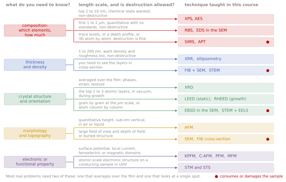
The course on one decision chart: start from the question, branch on the length scale and on whether the sample may be destroyed, and land on the technique.
Worked scenarios
The lecture develops several end-to-end scenarios; they make good exam practice.
An ALD hafnium oxide gate stack shows higher leakage after a process change. (Thickness and density: XRR and ellipsometry. Chemistry and interfacial layer: XPS. If localized: c-AFM to find hot spots, FIB and STEM-EELS at one.)
A sputtered metal interconnect film delaminates intermittently. (Interface chemistry: XPS or AES on both delaminated faces. Stress: wafer curvature and XRD. Morphology: SEM/EBSD for texture and boundaries.)
A perovskite solar absorber degrades under illumination. (GIWAXS for phase evolution, PL mapping for defect activity, ToF-SIMS for ion migration, cryo-STEM only with a careful dose budget.)
References and further reading
C. R. Brundle, C. A. Evans, and S. Wilson (eds.), Encyclopedia of Materials Characterization, Butterworth-Heinemann (1992).
D. K. Schroder, Semiconductor Material and Device Characterization, 3rd ed., Wiley (2006).