

A surface is a defect. Terminating a crystal removes the bonding partners of every atom in the outermost layers, and the material responds: surface atoms relax, reconstruct, adsorb whatever the environment offers, and trade places with atoms from the bulk. Every technique in this course exists because the composition and structure of the top few nanometers of a material routinely differ from the bulk, and because those few nanometers control adhesion, catalysis, corrosion, contact resistance, nucleation, and the behavior of essentially every interface in a device.
We start with the single most important concept of the module, surface energy, built up first in a two-dimensional model simple enough to play with, then stated properly in three dimensions.
Surface energy in two dimensions
Atoms in this model interact through the Lennard-Jones pair potential,
where is the separation of two atoms, is the depth of the energy minimum, and is the separation at which the potential crosses zero. The term is the repulsion of overlapping electron clouds and the term is the attractive van der Waals tail. The minimum sits at
so is the equilibrium bond length and is the bond strength. The total energy of a configuration of atoms is the sum over distinct pairs,
with the distance between atoms and . The simulation truncates the potential at , so each atom feels its nearest neighbors strongly and the next shell weakly.
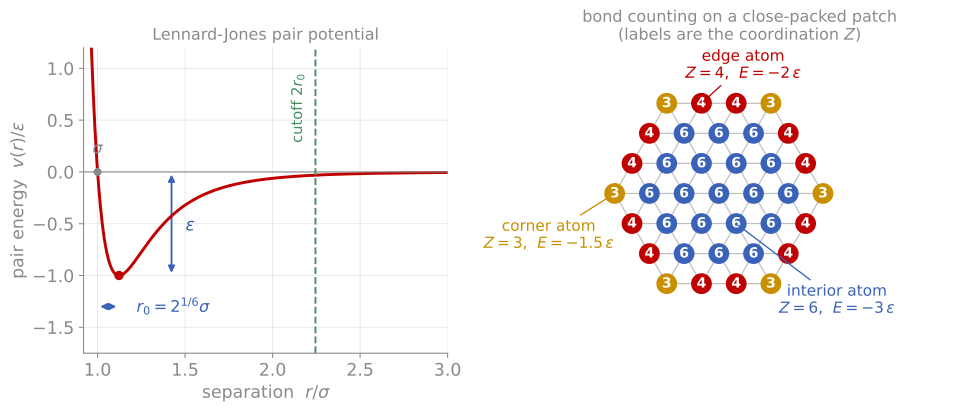
The Lennard-Jones potential and the bond counting it produces. Left: the pair energy , with the well depth , the zero crossing , the equilibrium bond length , and the cutoff used in the simulation. Right: a 37-atom close-packed patch labeled by coordination number . Interior atoms have , atoms on a straight close-packed edge have , and the six corners have .
Bond counting follows from the potential. If every neighbor sits at and everything beyond the first shell is neglected, each bond contributes , and each bond is shared between two atoms, so an atom with coordination number carries
The two-dimensional close-packed lattice has , giving the bulk value per atom. An atom on a straight close-packed edge keeps and costs , a corner atom keeps and costs , and an isolated atom costs nothing. Each edge atom therefore sits above the bulk value, and with edge atoms spaced apart the energy per unit length of a straight edge is
the two-dimensional analogue of the surface energy, measured in energy per length rather than energy per area.
The 37-atom patch in the figure works the example through. It has 19 interior atoms, 12 edge atoms, and 6 corner atoms, so
against a bulk reference of . The difference, , is the surface energy of the patch, and it is 19% of the bulk energy for a crystal only seven atoms across. Dividing by the perimeter of 18 bond lengths gives , slightly above the straight-edge value because the corners are more undercoordinated than the edges. Writing the total as
with the perimeter, shows the general result: a compact patch has , so the surface term falls only as and stays significant to large sizes. Everything else on this page follows from atoms rearranging to reduce this term.
Surface energy sandbox
The simulation below simulates example surfaces in two dimensions. Atoms evolve by Langevin dynamics at a temperature you control with the slider, and are colored by their energy: interior atoms sit at the bottom of the scale and appear dark, while undercoordinated atoms at surfaces, edges, corners, and grain boundaries glow. The box is periodic, so nothing is lost off the edges.
Some experiments worth performing, roughly in order:
Stability. The hexagon is the equilibrium shape and simply vibrates. The triangle and snowflake have the same kind of atoms but more perimeter per atom; check their energies against the hexagon in the right panel.
Metastability. The square lattice is not the ground state, yet when cold it persists indefinitely: there is an energy barrier between it and the close-packed lattice. Warm it and it shears into close packing. The quasicrystal, a twelve-fold square-triangle tiling, is built entirely from these two locally stable motifs and likewise holds together cold, transforming only slowly when warmed; the ring teaches the same lesson in shape form. This distinction between the lowest-energy state and the states that survive kinetically appears throughout thin film science.
The limits of pair bonding. The honeycomb, the open network of graphene, collapses even when cold: a three-coordinated network is floppy under central pair forces no matter how the interaction range is chosen. Watching it crumple is the demonstration of why real 2D materials depend on directional covalent bonds, which resist bending in a way no pair potential can.
Surface diffusion. At moderate temperature, edge atoms hop along the perimeter far more readily than anything moves in the interior. This is why annealing works: the snowflake’s arms retract into a compact hexagon by edge diffusion alone.
Sintering and ripening. The pair of touching particles forms a neck that thickens as the two coalesce, eliminating surface. It is slow when cold, because coalescence is limited by the same surface diffusion; warm it gently and watch the neck grow. The islands preset scatters particles of many sizes, the morphology of an early-stage deposited film: warmed, the small islands lose atoms to the large ones.
Grain boundaries. The bicrystal and the two dense polycrystal presets fill the box completely, so the only defects are the internal interfaces. The boundary atoms glow for exactly the same reason edge atoms do: missing and misaligned bonds. Start with the bicrystal to see a single boundary cleanly, compare the energy per atom of coarse and fine grains, then warm the fine-grained sample and watch boundaries move.
Phases. The gas preset starts hot. Cool it through roughly to 0.4 and a liquid droplet condenses from the vapor; cool further and it crystallizes. Quench fast versus slow and compare the crystals you get. The glass preset is the other endpoint: a jammed amorphous packing of two atom sizes that flows when warmed but resists crystallizing, the structure of an amorphous thin film.
Defects by hand. Drag atoms to build vacancies, adatoms, or notches, and watch them heal, or fail to heal if it is cold. The notch preset seeds a sharp crack for you; warm it and watch the tip blunt.
The energy trace in the right panel is the quantitative summary: every spontaneous change moves it downhill, and each discrete step is one rearrangement event.
Surface energy in three dimensions
Nothing changes in three dimensions except the bookkeeping. The two-dimensional argument had three steps: count the bonds a surface atom has lost, convert that count into an energy using the bond strength, and divide by the size of the boundary. Take the same three steps with an area in place of a length.
An atom that has lost of its bonds carries half the energy of each broken bond, because a bond belongs equally to the two atoms it joins, so it sits
above a bulk atom, where is the number of bonds broken per surface atom and is the bond strength, meaning the energy needed to break one bond completely.
The bond strength is not usually tabulated, but the cohesive energy is. A crystal of atoms with neighbours each contains bonds rather than , because every bond is shared by the two atoms it joins, so the binding energy per atom is
where is the cohesive energy per atom and is the bulk coordination number. Substituting, and dividing the excess energy by the area that each surface atom occupies, gives the surface energy
The two factors of two cancel, and no factor of a half survives into the result. They are the same rule applied in opposite directions: the first splits each broken bond between the two surfaces the cut creates, and the second undoes the sharing that made the cohesive energy per atom rather than . What is left says that a surface atom costs the same fraction of the cohesive energy as the fraction of its bonds it has lost, which is of for fcc (111), and that sentence can be written down without counting halves at all.
The two-dimensional result is this same expression with a length in place of the area. There , an edge atom loses bonds, , and the boundary per atom is rather than , which returns , the line tension found above.
The quantity this estimates is defined thermodynamically as the reversible work required to create a unit area of new surface,
where is the Gibbs free energy of the system in J, is the surface area in m, and the subscripts fix the temperature , the pressure , and the number of atoms of each species while the area is changed. The units are J/m, equivalently N/m, and values are often quoted in mJ/m.
Applying the estimate to a real crystal face needs two numbers, and the geometry of the plane gives both: how many bonds the cut breaks, and how closely the surface atoms are packed.

Bond counting on the three low-index fcc surfaces, drawn in cross-section with the broken bonds as stubs. The more open the plane, the more bonds each surface atom loses and the more area it occupies. The bar chart evaluates for copper, with , eV per atom, and nm.
Worked example: cleaving diamond
Cleaving splits the crystal along a plane, breaking every bond that crosses it, and the energy is shared between the two new surfaces that appear:
where is the number of surface atoms per unit area in m, is the number of bonds each of those atoms loses, is the bond energy in J, and the factor of one half divides the work between the two faces.
Diamond has the cubic lattice parameter nm, bulk coordination , and cohesive energy eV per atom, so the bond energy is
close to the tabulated C-C single-bond dissociation energy of about 3.6 eV. For the (111) plane, the surface atom density is
which is atoms/cm, and the (111) cut passes through the single bond that points along the surface normal, so . Putting the three numbers together,
Measured cleavage energies for diamond (111) fall between about 5 and 6 J/m.
The (100) plane is more open, m, and the cut passes through two bonds per surface atom, :
1.7 times the (111) value. Both numbers are far larger than every entry in the table below, which is why diamond is hard to cleave and why its surfaces reconstruct strongly, and the factor of 1.7 between the two planes is why cleavage selects (111).
The same bond count predicts a correlation with the heat of sublimation. The heat of sublimation is the energy needed to take one mole of atoms from the solid straight into the vapor, which breaks every bond each atom has:
with the Avogadro constant, so it is the cohesive energy per mole. A surface breaks of those bonds instead of all of them, so the surface energy per atom is the fraction of the sublimation energy per atom, typically one quarter to one half. Measured surface energies plotted against tabulated heats of sublimation follow that line across the periodic table. This is useful in practice: sublimation heats are tabulated for everything and surface energies are not, so when a is missing the sublimation heat gets within tens of percent.

Surface energy tracks sublimation. For representative metals: the same bonds are broken partially by a surface and completely by sublimation, so the two track each other. Values are approximate.
This crude estimate captures both the magnitudes and the trends: surface energy scales with cohesive energy, so bond type organizes the table. Van der Waals solids sit lowest, hydrogen-bonded liquids next, then oxides, then metals in proportion to their cohesion, and covalent networks highest. Representative values, sorted by :
| Material | Bonding | (J/m) |
|---|---|---|
| PTFE | van der Waals | 0.02 |
| Polyethylene | van der Waals | 0.03 |
| Water (liquid) | hydrogen bonding | 0.07 |
| SiO (fused silica) | oxide | 0.26 |
| TiO (110, rutile) | oxide | 0.44 |
| Mercury (liquid) | metallic | 0.49 |
| Pb | metallic | 0.60 |
| Mg | metallic | 0.79 |
| Al | metallic | 1.1 |
| MgO (100) | oxide | 1.2 |
| Si (111) | covalent | 1.2 |
| Ag | metallic | 1.3 |
| AlO (0001) | oxide | 1.4 |
| Au | metallic | 1.5 |
| Cu | metallic | 1.8 |
| Ti | metallic | 2.1 |
| Fe | metallic | 2.4 |
| Ni | metallic | 2.4 |
| Pt | metallic | 2.5 |
| Mo | metallic | 3.0 |
| W | metallic | 3.7 |
| Diamond (111) | covalent | about 5.7 |
The metal and oxide pairs in that table decide whether a native oxide spreads. Three energies are involved: for the clean metal surface, for the buried metal-oxide interface, and for the oxide surface. A continuous oxide film removes the metal surface and creates two new boundaries in its place, so it lowers the total energy when
Silicon and titanium satisfy this with room to spare, since alone is four to five times below , and their oxides wet the metal completely rather than balling up into islands. That is why native oxides are continuous and passivating, and why the surface measured on any air-exposed metal is an oxide surface unless it was cleaned in vacuum. Aluminium is the case to watch: a clean AlO surface is not far below clean aluminium, and it is the hydroxyl and adsorbate coverage that any oxide picks up in air that lowers enough.
Solid surface energies are measured only with difficulty (typically from high-temperature zero-creep experiments or liquid-metal extrapolations) and calculated values differ between methods, so treat any single number as approximate; the values above follow the compilations of Tyson and Miller (Tyson & Miller (1977)) and the calculations of Vitos et al. (Vitos et al. (1998)). Wikipedia’s surface energy article maintains a longer table with sources.
Because depends on orientation, a crystal free to choose its shape minimizes total surface energy rather than total area, giving the faceted equilibrium shapes of the Wulff construction, exactly the physics that turned the simulated disk into a hexagon. Surface energy balances also decide whether a deposited film wets its substrate or balls up into islands, set the driving forces for grain growth and sintering, and drive the segregation and adsorption phenomena below.
Wulff construction
The construction below computes both cases. On the left, the polar plot of and the equilibrium shape it generates: with no anisotropy the shape is a circle (a liquid drop), and as anisotropy grows, facets appear and sharpen. On the right, the Winterbottom extension puts the same crystal on a substrate: the balance of surface, interface, and substrate energies truncates the shape, and sweeping the wetting parameter moves the island continuously from a barely attached particle to a spread film. This is the equilibrium framework behind island growth, dewetting, and why deposited films ball up on substrates they do not wet.
Terraces, steps, and kinks
Real surfaces are not single perfect planes. A surface cut slightly off a low-index orientation (a vicinal surface) decomposes into low-energy terraces separated by atomic steps, with the step spacing set by the miscut angle; the steps themselves contain kinks. This terrace-step-kink picture organizes almost everything kinetic that happens on a surface. Kink sites are special: an atom attaching or detaching at a kink leaves the kink itself unchanged, so the kink is the repeatable growth site, and its energy sets the equilibrium between a crystal and its vapor. Steps are where deposited atoms attach during growth and where atoms detach during evaporation and etching, which is why growth and dissolution both proceed by steps flowing across terraces rather than by atoms landing at random. The step and kink energies are the one- and zero-dimensional analogues of the surface energy, and the simulation above displays all three: facets (low energy, dark), step edges along the facets (brighter), and kink and corner atoms (brightest of all).
A related distinction worth keeping precise: the surface energy is the work to create new area (by cleaving), while the surface stress is the work to elastically stretch existing area. For liquids the two are equal, because a stretched liquid surface immediately repopulates with atoms; for solids they differ, and surface stress is what bends micromechanical cantilevers when molecules adsorb on one face.
Relaxation and reconstruction
The atoms at a real surface do not sit at truncated bulk positions. In relaxation, the surface layers keep the bulk periodicity parallel to the surface but shift perpendicular to it; the first interlayer spacing of most metal surfaces contracts by a few percent. In reconstruction, the surface adopts a different two-dimensional periodicity altogether to reduce the number of dangling bonds. The canonical example is Si(111) 7x7, a reconstruction whose unit cell contains 49 original surface cells and whose structure took a quarter century and the invention of scanning tunneling microscopy to solve. Semiconductors reconstruct strongly because their bonds are directional and dangling bonds are expensive; metals reconstruct less often.
Reconstructions matter to us for two reasons. They change surface reactivity and epitaxial growth behavior, and they produce the superstructure spots we will learn to read in low-energy electron diffraction in Module 6.
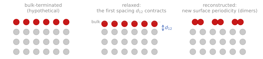
Relaxation and reconstruction. The three responses of a terminated crystal: hypothetical bulk termination, relaxation of the first interlayer spacing, and reconstruction into a new surface periodicity, drawn here as dimer rows of the kind Si(100) forms.
Adsorption and the need for vacuum
A surface in any real environment is being bombarded by gas molecules. The flux of molecules striking a surface follows from the kinetic theory of gases,
where is the number of molecules striking unit area per unit time, is the pressure, is the mass of one molecule, is the Boltzmann constant, and is the temperature. At atmospheric pressure this flux is about molecules per cm per second for nitrogen, enough to deliver a complete monolayer in a few nanoseconds if every molecule stuck. Even at 10-6 Torr, a good high vacuum, a monolayer arrives roughly every second. Keeping a surface atomically clean for the duration of an experiment, one hour say, requires pressures near 10-10 Torr. This single estimate explains why surface analysis instruments are built around ultrahigh vacuum, and we treat the technology on the next page.
Adsorption itself comes in two flavors. Physisorption binds molecules weakly through van der Waals forces, with binding energies below about 0.3 eV; chemisorption forms true chemical bonds, with energies of 1 eV or more. The residence time of an adsorbed molecule scales as with a vibrational period of order 10-13 s, so modest temperature changes swing surface coverage by orders of magnitude: a physisorbed molecule at room temperature leaves almost immediately, while a chemisorbed one is effectively permanent.
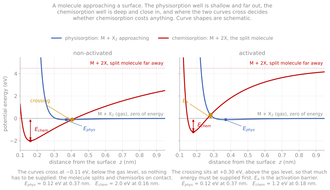
Physisorption and chemisorption as one-dimensional potentials. Where the two curves cross sets whether chemisorption is activated: below the gas level the molecule dissociates on contact, above it there is a barrier to pay.
The simplest quantitative model of equilibrium coverage is the Langmuir isotherm: assume a fixed number of equivalent sites, one molecule per site, and no interactions between adsorbates. Balancing the arrival rate (proportional to pressure, from the flux formula above, times the fraction of empty sites) against the thermally activated desorption rate gives a coverage
where is the fraction of sites occupied, is the pressure, and is the adsorption equilibrium constant, which carries the binding energy and the temperature. The coverage rises linearly at low pressure and saturates at one monolayer. Real systems decorate this picture with adsorbate interactions, multilayer condensation, and site heterogeneity, but the Langmuir form remains the working baseline.
An isotherm is measured at one fixed temperature, which is what the word means, and it says where the coverage settles rather than how long it takes to get there. How fast a clean surface fills is the separate kinetic question, and surface science quotes it as an exposure, pressure times time, in langmuir: 1 L is 10-6 Torr for 1 s, which at unit sticking delivers molecules per cm, so one langmuir is roughly one monolayer. That is the monolayer-time arithmetic of the next page in different units.

Left: the Langmuir isotherm at three adsorption energies, saturating at one monolayer with half coverage at . Right: coverage against exposure in langmuir, for three sticking coefficients.
Temperature-programmed desorption measures binding energies directly. Dose a cold surface with a known exposure, then heat it at a constant rate while a mass spectrometer records what leaves; each bound state empties over a narrow temperature window and appears as a peak, so several peaks mean several distinct binding sites. The peak temperature fixes the desorption energy through the Redhead relation, which for first-order desorption is
with the desorption energy, the peak temperature, the heating rate in K/s, s the attempt frequency, and the Boltzmann constant. The rule of thumb that follows is about 2.7 meV of binding per kelvin of peak temperature, so a peak at 300 K means roughly 0.8 eV. The area under the peak gives the coverage that was there.
Adsorbed atoms also move. Surface diffusion is thermally activated hopping between sites, with barriers typically a few tenths of an electron-volt on close-packed metal terraces, far below bulk diffusion barriers; this is why surfaces equilibrate at temperatures where bulks are frozen, and why every annealing behavior in the simulation above is dominated by atoms skating along edges rather than moving through the interior. One subtlety with large consequences for film growth: an atom approaching a descending step often faces an extra barrier to hopping down over the edge (the Ehrlich-Schwoebel barrier), which traps atoms on top of islands and can tip growth from smooth layer-by-layer toward three-dimensional mounds, a kinetic effect we will meet again in the RHEED discussion of growth modes.

Diffusion across a terrace against stepping down off an island, with the energy landscape drawn under the atoms. Hopping along the terrace pays the terrace barrier each time, while crossing the descending edge pays the Ehrlich-Schwoebel barrier on top of it, which traps atoms on the island and tips growth toward mounds.
Segregation
The composition of a surface is not the composition of the bulk. In an alloy, the component that lowers the total energy, generally the one with the lower surface energy or the larger size mismatch, enriches at the surface. The equilibrium enrichment follows Boltzmann statistics: moving an atom to the surface costs the fraction of its bonds that a surface site lacks, so each species distributes as
where and are the concentrations of that species at the surface and in the bulk, is the fraction of bonds a surface site lacks, is the sublimation energy per mole of that species, is the gas constant, and is the temperature. The species with the smaller sublimation energy, which is the lower- component, segregates to the surface. Because the energies in the exponent are electron-volts against a thermal energy of hundredths of an electron-volt, the enrichment factors are large: segregation of a dilute impurity can be dramatic, and a bulk concentration of parts per million can produce near-monolayer surface coverage at equilibrium. Segregation also takes time, and the kinetics are set by bulk diffusion. For arrival at an initially clean surface, the surface excess after a time is
where is the number of segregated atoms per unit area, is the bulk concentration per unit volume, is the bulk diffusion coefficient, and is the time at temperature. The structure is concentration times the diffusion length : the surface collects everything within a diffusion length of it, so a ppm impurity can reach a tenth of a monolayer during a routine anneal, and any heat treatment inside the analysis chamber changes the surface you were about to measure. :::{figure} ../../assets/figures/segregation-kinetics.svg :alt: equilibrium enrichment against temperature, and coverage building as the square root of time :width: 100%
Left: the equilibrium enrichment of the Boltzmann form above, which falls as the temperature rises. Right: the diffusion-limited buildup for 5 ppm sulfur in nickel, which reaches a tenth of a monolayer in about 25 minutes at cm/s.
This is the working principle behind temper embrittlement of steels, the poisoning of catalysts, and many adhesion failures. It is also a warning for us as analysts: a technique that samples the top one or two atomic layers, such as low-energy ion scattering or grazing-emission XPS, can report a composition very different from the bulk, and both numbers are correct.

## The electronic surface

The electronic structure also changes at the surface. The conduction electron density of a metal does not stop abruptly at the last atomic plane: it spills a fraction of an angstrom into the vacuum and, inside the crystal, relaxes back toward the bulk density through decaying (Friedel) oscillations. The spillout separates negative charge from the positive ion cores, creating a surface dipole layer that every escaping electron must cross.

The **work function** $\phi$ is the energy needed to take an electron from the Fermi level of the solid to rest in the vacuum just outside the surface, a few eV for a metal. Part of it is bulk, the chemical potential of the electrons, and part is the work done crossing that dipole, which is what makes $\phi$ a surface property rather than a bulk one: different facets of the same metal differ by up to about 1 eV because they pack differently and so spill differently. An adsorbate that donates charge to the metal shrinks the dipole and lowers $\phi$, and one that withdraws charge raises it; submonolayer caesium drops the work function of tungsten by more than 2 eV, which is how thermionic cathodes are made.

On a semiconductor the broken bonds at the surface leave electronic states in the band gap, and those states trap charge until the Fermi level at the surface sits at a fixed position in the gap. That is **Fermi level pinning**, and it is why a metal contact on many semiconductors gives a barrier height that hardly depends on which metal is used. The same dangling bonds drive the reconstructions above, because pairing them into dimers removes states from the gap and lowers the energy. :::{figure} ../../assets/figures/electron-spillout.svg
:alt: electron density across a metal surface, showing spillout and the dipole layer
:width: 100%

The electron density across a metal surface. The electrons leak past the edge of the positive background, leaving a charge deficit just inside and an excess just outside, and that pair is the surface dipole every escaping electron must cross. Inside, the density rings as it settles to the bulk value.
These electronic differences matter directly for characterization: they set the contrast mechanism of scanning tunneling microscopy, the signal of Kelvin probe microscopy, and the reason work functions appear throughout the electron spectroscopies of Module 4.
The analytical puzzle
Every characterization problem in this course reduces to the same set of questions:
What do you want to know? Composition, chemical bonding state, crystal structure, thickness, roughness, morphology, defect content, or a depth profile of any of these.
Where is the information? The top atomic layer, the top few nanometers, a buried interface, or the full film.
What resolution and sensitivity do you need? Lateral resolution from millimeters to angstroms, detection limits from percent to parts per billion.
What can the sample tolerate? Vacuum exposure, electron or ion beam damage, the destruction of the analyzed region, or the effort of preparing a thin cross-section.
No single technique answers all of these at once. XPS gives chemical states but averages over a large spot; atom probe gives three-dimensional composition with atomic resolution but destroys the sample; STEM sees a buried interface directly but only after the interface has been cut out and thinned. Learning the strengths and limits of each technique, well enough to design a characterization strategy for a problem you have never seen before, is the goal of this course. We return to this puzzle explicitly in the final synthesis lecture.
References and further reading
A. Zangwill, Physics at Surfaces, Cambridge University Press (1988), Chapters 1 to 4.
K. Oura et al., Surface Science: An Introduction, Springer (2003), Chapters 1, 10, and 14.
L. C. Feldman and J. W. Mayer, Fundamentals of Surface and Thin Film Analysis, North-Holland (1986), Chapter 1.
W. R. Tyson and W. A. Miller, Surface free energies of solid metals: estimation from liquid surface tension measurements, Surface Science 62, 267 (1977). Tyson & Miller (1977)
L. Vitos, A. V. Ruban, H. L. Skriver, and J. Kollár, The surface energy of metals, Surface Science 411, 186 (1998). Vitos et al. (1998)
G. Binnig, H. Rohrer, Ch. Gerber, and E. Weibel, 7x7 reconstruction on Si(111) resolved in real space, Physical Review Letters 50, 120 (1983). Binnig et al. (1983)
Surface energy on Wikipedia, including its table of measured surface energies.
- Tyson, W. R., & Miller, W. A. (1977). Surface free energies of solid metals: Estimation from liquid surface tension measurements. Surface Science, 62(1), 267–276. 10.1016/0039-6028(77)90442-3
- Vitos, L., Ruban, A. V., Skriver, H. L., & Kollár, J. (1998). The surface energy of metals. Surface Science, 411(1–2), 186–202. 10.1016/s0039-6028(98)00363-x
- Binnig, G., Rohrer, H., Gerber, Ch., & Weibel, E. (1983). 7 × 7 Reconstruction on Si(111) Resolved in Real Space. Physical Review Letters, 50(2), 120–123. 10.1103/physrevlett.50.120