
The atomic force microscope maps a surface by touch. A tip a few nanometers sharp, mounted on a flexible cantilever, is scanned across the sample while a feedback loop holds the tip-sample interaction constant; the feedback signal traces out topography with sub-angstrom height resolution. No vacuum, no conductivity requirement, no sample preparation: AFM images metals, oxides, polymers, and wet biological samples equally well, which is why it sits in nearly every materials laboratory and cleanroom. For thin films AFM is the standard measurement of surface roughness, and its quantitative use is the subject of this page.
| At a glance | |
|---|---|
| Probe in / signal out | Sharp tip on a cantilever in mechanical interaction with the surface |
| Information | Topography, roughness statistics, step heights, grain morphology; mechanical properties |
| Vertical resolution | Better than 0.1 nm; atomic steps trivially resolved |
| Lateral resolution | 1 to 10 nm, set by tip radius |
| Field of view | Up to about 100 um; scan times of minutes |
| Sample requirements | Any reasonably smooth solid, in air, liquid, or vacuum; nondestructive |
The transducer
The cantilever is a calibrated spring: forces between tip and sample of piconewtons to nanonewtons deflect a cantilever of stiffness from about 0.01 N/m (soft contact levers) to about 40 N/m (stiff tapping levers), and the deflection is read out by a laser reflected off the cantilever’s back onto a split photodiode. The optical lever multiplies angular deflection by the beam path length, converting sub-angstrom motions into measurable photocurrent differences: mechanical amplification with no contact and negligible noise, the enabling trick of practical AFM. Oscillating modes add the cantilever’s resonance, , typically tens to hundreds of kHz, whose amplitude, phase, and frequency become measurement channels. Quantitative work calibrates both conversion factors rather than trusting nominal values: the deflection sensitivity from a force curve on a hard surface, and the spring constant most conveniently from the cantilever’s thermal vibration spectrum (the equipartition theorem turns the measured Brownian motion into ), the standard “thermal tune.”
A force-distance curve, deflection versus tip approach, is the technique’s central calibration and diagnostic tool: approaching from far, the tip feels growing van der Waals attraction until the force gradient exceeds and the tip snaps into contact; pressing further climbs the repulsive wall; retracting shows adhesion hysteresis before snap-off, with the pull-off force measuring tip-sample adhesion (interpreted through contact mechanics models when quantitative adhesion or modulus is the goal). Everything about imaging modes follows from where on this curve the instrument operates.
Imaging modes
Contact mode drags the tip in repulsive contact at constant deflection (constant force). Simple and fast, and the mode of choice for friction measurements (lateral force microscopy reads the cantilever’s twist), but lateral forces damage soft samples and dull tips.
Tapping mode (amplitude-modulation AFM) oscillates the cantilever near resonance with tens of nanometers amplitude; intermittent contact reduces the amplitude, and the feedback holds that reduced amplitude constant. Lateral forces nearly vanish, which is why this is the default mode for most work. The phase of the oscillation relative to the drive is a free second channel: phase lag maps energy dissipation per tap, often revealing compositional contrast in polymer blends and contamination invisible in topography. One operational subtlety worth knowing: the oscillating tip can sit in a net-attractive or net-repulsive regime, and bistable switching between them mid-image produces artifacts cured by adjusting amplitude and setpoint.
Frequency-modulation (non-contact) AFM tracks the resonance frequency shift caused by the force gradient, without touching; in UHV with careful technique this achieves true atomic resolution, and with CO-functionalized tips at cryogenic temperature it famously resolves the internal bond architecture of single molecules.
Force-curve mapping modes record a complete force-distance curve at every pixel at kHz rates, extracting topography, modulus, adhesion, and deformation simultaneously, the quantitative-nanomechanics workhorse for polymers and composites.
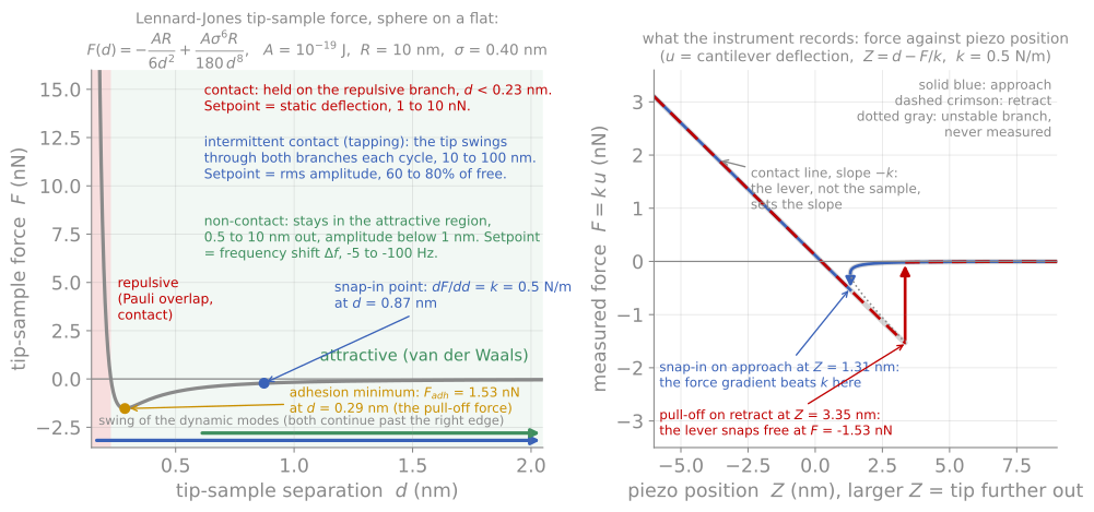
Module 7 in one figure. Every scanning probe mode is a choice of what to hold constant on this curve, or of what second quantity to record alongside the height.
Quantitative roughness metrology
The AFM’s headline number for thin films is roughness, and using it well takes more care than reading the RMS value off the screen. The standard statistics, average roughness and RMS roughness (the standard deviation of heights), characterize the height distribution only; two surfaces with identical can be morphologically different, one gently undulating, one sharply jagged. The power spectral density (PSD) of the height map resolves roughness by lateral wavelength, separating measurement noise, grain-scale texture, and long-range waviness, and is the right basis for comparing films or feeding roughness into optical and XRR models. Any reported roughness is a bandwidth-limited quantity: the scan size sets the longest wavelength included and the pixel spacing the shortest, so grows with scan size on most real surfaces, and a roughness value reported without its scan size is incomplete. Comparing an AFM against an XRR roughness, which averages a millimeter footprint with its own bandwidth weighting, requires exactly this thinking, and agreement within tens of percent is success.
Step-height measurement is the other precision use: an AFM profile across a masked or etched step measures film thickness absolutely, to sub-nanometer accuracy, with no optical model at all, which is why step-height standards calibrate the instrument’s z axis and why a deliberately patterned step is the fastest arbiter when ellipsometry and XRR disagree.

One surface measured two ways. The scan size sets the longest wavelength included and the pixel size the shortest, so without both numbers is not a measurement.
Artifacts
Tip shape simulation
Every AFM image is the interaction of two shapes: the surface and the tip. The demonstration below scans a realistic tip, an apex sphere blended into a conical shank, across known test structures, drawn at true aspect ratio so the shapes are not exaggerated. The tip presets carry representative radii and sidewall angles: a standard Si probe, a very sharp SiN probe, and a blunt diamond-coated probe for conductive or wear-heavy work. Sweep the radius on the particles preset and watch every feature broaden as roughly while heights stay correct; try the trench, where the sidewall angle, not the radius, decides whether the floor is reachable; and enable the double tip for the characteristic ghost-image doubling artifact. The measured is always at or below the true value, because the tip is a low-pass filter.
Other artifacts
Beyond tip shape, the standard artifact checklist: feedback ringing on steep edges (visible as overshoot on one side), thermal drift and piezo creep skewing slow scans, scanner bow adding false long-wavelength curvature, and the line-by-line leveling that every AFM image receives, which is necessary (each scan line has an arbitrary offset) but can erase real long-wavelength structure or create streaks from particles dragged by the tip. The working rules are simple: know the tip condition (image a known sharp standard when in doubt), image the same area twice with the scan rotated, and treat any feature at the resolution limit with suspicion.
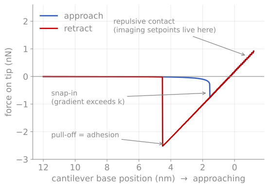
The force-distance curve. A computed cycle (van der Waals attraction plus contact repulsion against a 0.6 N/m lever): snap-in where the force gradient exceeds the spring constant, the repulsive regime used for imaging setpoints, and the pull-off event that measures adhesion.
References and further reading
B. Voigtländer, Atomic Force Microscopy, 2nd ed., Springer (2019). The modern instrument-level treatment.
F. J. Giessibl, Advances in atomic force microscopy, Reviews of Modern Physics 75, 949 (2003). Giessibl (2003)
G. Binnig, C. F. Quate, and Ch. Gerber, Atomic force microscope, Physical Review Letters 56, 930 (1986). Binnig et al. (1986)
- Giessibl, F. J. (2003). Advances in atomic force microscopy. Reviews of Modern Physics, 75(3), 949–983. 10.1103/revmodphys.75.949
- Binnig, G., Quate, C. F., & Gerber, Ch. (1986). Atomic Force Microscope. Physical Review Letters, 56(9), 930–933. 10.1103/physrevlett.56.930