
A focused sub-angstrom probe positioned on a chosen atomic column can do more than image. The inelastic signals developed in electron-solid interactions, energy losses and characteristic X-rays, are generated at the probe position and collected in parallel with every image, making the STEM a spectroscopy platform with the best spatial resolution of any technique in this course. Analytical STEM maps composition and chemical bonding across interfaces atom column by atom column, and for thin film problems it is the final arbiter: when depth profiles from sputter-based techniques disagree, a STEM-EELS line profile across the actual interface settles the question.
STEM-EELS
The electron energy loss spectrometer sits after the sample: a magnetic prism bends the transmitted beam, dispersing it by energy exactly as a glass prism disperses light, and a fast detector records the spectrum. Everything about the loss spectrum carries over from the earlier discussion; what the STEM adds is position. Recording a spectrum at every probe position of a scan (a spectrum image) turns each spectral feature into a map, and the modes divide by energy range:
Core-loss edges map elemental composition with atomic resolution. Quantification integrates each edge above its extrapolated background (fitted as a power law in the region before the edge) and divides by a calculated partial ionization cross section, yielding areal densities and elemental ratios to roughly 5 to 10% relative accuracy. The light elements (Li, B, C, N, O), which EDS measures poorly, have sharp accessible K edges that EELS measures well.
Energy-loss near-edge structure (ELNES) maps bonding: the shape of an edge within a few tens of eV of threshold reflects the local unoccupied density of states. The workhorse examples are canonical: transition-metal L/L “white line” intensity ratios track d-band filling and hence oxidation state (the Mn and Ti valence maps of oxide-interface science), the O K edge fingerprints coordination chemistry, and the C K edge’s / structure separates sp from sp carbon. This is chemical-state information of the same kind XPS provides, at a thousand times finer spatial scale, though with a harder quantification path.
Low-loss spectra measure the local dielectric response: plasmon energies track valence electron density (and, through it, composition and even local mechanical properties in some alloys), band gaps can be read from the loss onset in insulators, and surface-plasmon modes of nanostructures are mapped directly. The low-loss region also provides the standard thickness measurement: the probability of plasmon losses is Poissonian, so gives thickness in units of the inelastic mean free path from a single spectrum, the routine normalization for quantitative work.
Monochromated instruments narrow the beam’s energy spread to a few meV, extending EELS to phonons and molecular vibrations, vibrational spectroscopy at nanometer scale, a capability that did not exist before 2014.
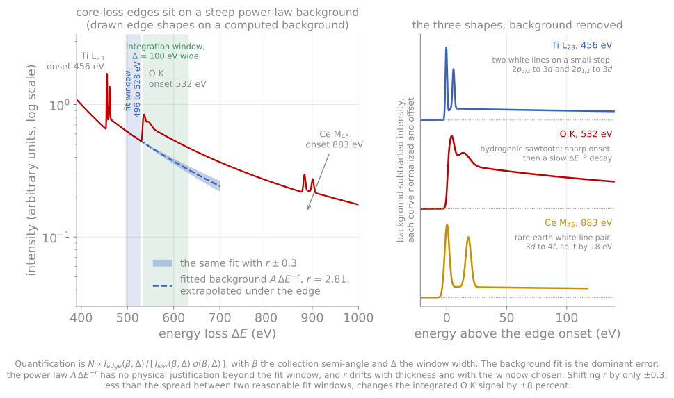
Three edge shapes on the same falling background, with the power-law fit window, the extrapolated background, and the integration window drawn on the O K edge. Shifting the fitted exponent by only 0.3 moves the integrated signal by 8%.
The constraints are dose and thickness. Core-loss cross sections are small, so atomic-resolution chemical maps push against beam damage, and samples much thicker than about one inelastic mean free path (roughly 100 nm at typical conditions) bury the edges under multiple scattering (“plural scattering”), correctable in part by deconvolution but best avoided: thin, well-prepared samples are not optional for EELS.
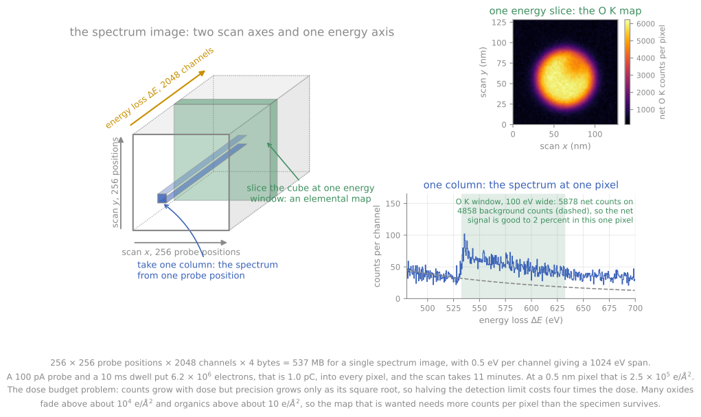
One energy slab through the cube is an elemental map and one column is a spectrum. The numbers on the figure are the dose budget: 537 MB, eleven minutes, and electrons per square angstrom.
STEM-EDS
The same characteristic X-rays used in SEM-EDS are collected in STEM by large solid-angle silicon drift detectors placed close around the sample. Because the sample is a thin foil, the micrometer interaction volume of bulk EDS collapses to essentially the probe diameter plus modest beam broadening through the foil: nanometer-scale X-ray mapping. Thin-foil quantification also simplifies considerably, since the ZAF matrix corrections of bulk analysis largely vanish. The classical Cliff-Lorimer method converts intensity ratios to composition ratios with a single factor per element pair (), calibrated on standards; the modern zeta-factor method works with absolute intensities and measured beam current, handling absorption of soft X-rays within the foil self-consistently, which matters for light elements and thicker lamellae. One crystalline-sample subtlety inherited from dynamical diffraction: when the beam channels along atomic columns, X-ray production is enhanced on whichever sublattice the beam channels through, so quantitative EDS of zone-axis crystals either tilts slightly off axis or accounts for channeling explicitly.
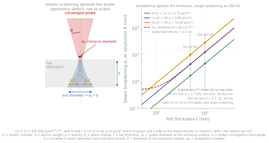
Elastic scattering spreads the probe as it crosses the foil, so the analysed volume is wider than the probe. Past about 15 nm of copper the probe size stops mattering and the thickness sets the resolution.
In modern practice STEM-EDS and STEM-EELS run simultaneously and are complementary: EDS covers heavy elements and full-stack overview maps with simple quantification and no thickness ceiling, EELS covers light elements, bonding, and the finest spatial detail. An elemental map of a complete device cross-section, every layer labeled, in under an hour, is now a routine measurement.
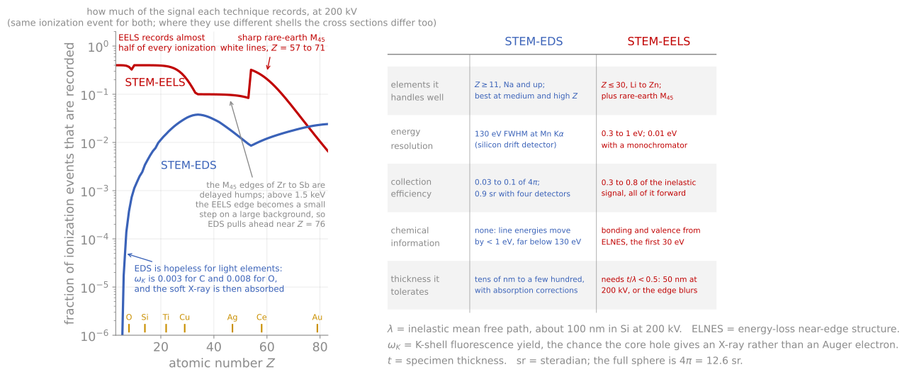
The fraction of ionization events each technique actually records, against atomic number, with the criteria side by side. EELS wins by four decades on the light elements and EDS pulls ahead near .
Strain and structure mapping
Diffraction-based STEM mapping completes the analytical picture. Scanning nanobeam diffraction tracks the positions of Bragg disks across the scan and converts their shifts to local lattice parameters, mapping the full two-dimensional strain tensor at a few nanometers resolution with about 0.1% precision, directly on the device feature of interest rather than averaged over a beam footprint as in X-ray methods. Geometric phase analysis extracts equivalent information from the lattice fringes of a single atomic-resolution image by Fourier filtering, fast and convenient where a good zone-axis image exists. For thin film development these maps answer whether the intended strain state survived patterning and processing, a question no ensemble technique can localize; their systematic errors (reference-region choice, projection through the foil, relaxation of the thin lamella itself, which partially releases the very strain being measured) are the caveats to carry into any quantitative claim.
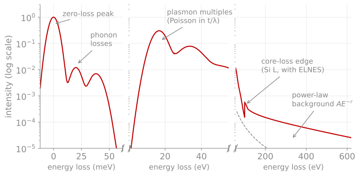
Anatomy of a loss spectrum. Phonon losses at the meV scale (accessible with a monochromator), the plasmon and its Poisson-distributed multiples, the falling background, and a core-loss edge carrying ELNES fine structure; the axis breaks step the energy scale from meV to eV. The plasmon-multiple statistics give the standard thickness measurement.
References and further reading
R. F. Egerton, Electron Energy-Loss Spectroscopy in the Electron Microscope, 3rd ed., Springer (2011). The definitive EELS reference, including all quantification formulas used here.
D. B. Williams and C. B. Carter, Transmission Electron Microscopy, 2nd ed., Springer (2009), Part 4 (spectrometry).
O. L. Krivanek et al., Vibrational spectroscopy in the electron microscope, Nature 514, 209 (2014). Krivanek et al. (2014)
- Krivanek, O. L., Lovejoy, T. C., Dellby, N., Aoki, T., Carpenter, R. W., Rez, P., Soignard, E., Zhu, J., Batson, P. E., Lagos, M. J., Egerton, R. F., & Crozier, P. A. (2014). Vibrational spectroscopy in the electron microscope. Nature, 514(7521), 209–212. 10.1038/nature13870