

X-ray diffraction is the first measurement made on nearly every crystalline thin film. It requires no vacuum, no sample preparation, and no contact, it averages over a statistically meaningful area, and a single afternoon of measurements can determine the phases present, the film texture, the strain state, and the crystalline quality. This page is self-contained: it builds up the diffraction physics from the scattering of X-rays by electrons, because the same reciprocal-space machinery returns later for LEED and RHEED and for electron diffraction in the STEM.
| At a glance | |
|---|---|
| Probe in / signal out | X-rays in, diffracted X-rays out |
| Information | Phase identification, orientation and texture, strain and stress, grain size, crystalline quality |
| Depth probed | Full film thickness; tunable from nanometers up using grazing incidence |
| Lateral resolution | Millimeters (lab); micrometers at synchrotrons |
| Sensitivity | Crystalline phases down to a few volume percent; film thicknesses down to a few nanometers with care |
| Sample requirements | Essentially none; measured in air, nondestructive |
X-rays and how they scatter
Laboratory X-rays come from a sealed tube: electrons accelerated through tens of kilovolts strike a metal anode, producing a continuous bremsstrahlung background plus intense characteristic lines emitted when a knocked-out core electron is replaced from a higher shell. The workhorse is the copper K line at Å (Cu K; the K companion at 1.5444 Å is either tolerated or removed with a monochromator, and the K line is removed with a Ni filter or monochromator). The wavelength matters because it is comparable to interatomic spacings, which is the entire reason X-ray diffraction exists. Synchrotron sources provide the same physics with orders of magnitude more flux, tunable wavelength, and micrometer beam sizes.
An X-ray scatters from the electrons of the sample: the oscillating electric field drives each electron, and the accelerating electron re-radiates at the same wavelength (Thomson scattering; this elastic channel is what diffraction uses). An atom scatters with an amplitude called the atomic form factor , equal to the number of electrons in the forward direction and falling off with scattering angle because the electron cloud has a size comparable to the wavelength. Two immediate consequences: heavy elements scatter X-rays more strongly, roughly as in amplitude and in intensity, and light elements (and especially hydrogen) are hard for X-rays to see, one of the recurring asymmetries between X-ray, electron, and neutron probes.
Diffraction from a crystal
A crystal is a periodic arrangement of atoms, and waves scattered from successive lattice planes interfere. For planes of spacing and X-rays incident at angle to those planes, the path difference between reflections from adjacent planes is ; constructive interference requires it to equal a whole number of wavelengths, which is Bragg’s law:
Here is the spacing of the planes, the angle between the beam and those planes, the order of the reflection, and the X-ray wavelength. Each set of lattice planes, labeled by Miller indices , has its own spacing (for a cubic crystal of lattice parameter , ) and therefore its own Bragg angle. A measured pattern of peak positions is thus a fingerprint of the lattice, and comparing measured positions and intensities against the powder diffraction database is how phases are identified.
The equivalent and more powerful statement is made in reciprocal space. Define the scattering vector , with for elastic scattering; its magnitude is . Diffraction occurs when equals a reciprocal lattice vector , a condition identical to Bragg’s law but which keeps track of directions as well as magnitudes. This picture, formalized as the Ewald sphere construction, is developed interactively in Module 6; for now the important habit is to think of every diffraction measurement as answering the question “which reciprocal lattice points does my scan pass through?”
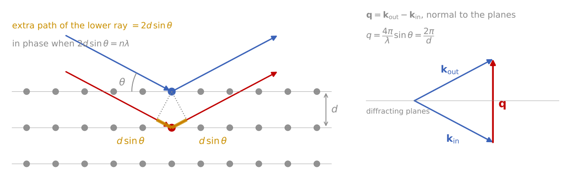
Bragg’s law and the scattering vector. Left: the ray scattered by the lower plane travels an extra , and the two rays add in phase when this equals a whole number of wavelengths. Right: the scattering vector points along the normal of the diffracting planes, with length at the Bragg condition.
Peak intensities carry as much information as positions. The scattering amplitude of one unit cell is the structure factor,
summing over the atoms in the unit cell at fractional positions , with the atomic form factor of atom , the amplitude that atom scatters, and the Miller indices of the reflection. Interference between atoms within the cell can cancel entire reflections: for an FCC metal, vanishes unless are all even or all odd, which is why an FCC powder pattern shows 111, 200, 220, 311 and nothing between. Measured intensities also fold in the number of symmetry-equivalent planes (multiplicity), the polarization and geometry-dependent Lorentz factor, thermal vibration (the Debye-Waller factor, which damps high-angle peaks), and absorption. Quantitative phase analysis and Rietveld refinement fit all of these at once; for thin film work the qualitative rules are usually enough: intensities scale with , and anomalies in relative intensities compared to the powder reference are the first sign of texture.
XRD pattern calculator
The calculator below turns this machinery into patterns. Pick a material and the reflections appear where the structure factor allows them: FCC copper shows 111 and 200, BCC tungsten shows 110, and diamond-cubic silicon is missing 200 and 222 entirely. Then add the microstructure of a real film: the texture slider narrows the pattern toward the single family of planes parallel to the surface (compare the two microstructure sketches), the grain-size slider broadens peaks by the Scherrer relation, and the microstrain slider broadens them with the signature that Williamson-Hall analysis exploits.
Instrumentation
The standard laboratory geometry is Bragg-Brentano (-): the source and detector move symmetrically so that stays perpendicular to the sample surface. It is parafocusing, meaning divergent illumination refocuses at the detector when the sample surface stays tangent to the focusing circle; the price is sensitivity to sample height error, which shifts peaks and is the most common alignment artifact in practice. Divergence slits set the illuminated length (and change it with angle, an intensity correction at low ), Soller slits limit axial divergence, and a monochromator or energy-resolving detector removes fluorescence background, important for Fe-containing samples with Cu radiation, where the Cu K beam efficiently excites Fe fluorescence. Modern instruments substitute a parallel-beam mirror plus a 1D strip detector, which relaxes the height-error sensitivity and speeds acquisition by orders of magnitude. High-resolution work adds a multi-bounce crystal monochromator on the incident side and an analyzer crystal on the diffracted side, at a large cost in intensity.
The thin film problem
A symmetric - scan of a film on a substrate has two difficulties. The substrate, being vastly thicker, dominates the pattern with intense peaks that can bury the film signal, and for a strongly textured or epitaxial film only the lattice planes parallel to the surface diffract at all, so most of the pattern is simply absent. Once understood, both effects become measurement tools. The substrate peaks provide an internal calibration for the film peak positions, and the presence or absence of film reflections is itself a measurement of orientation.
For polycrystalline films the standard fix is grazing incidence XRD (GIXRD): the incident beam is fixed at a small angle of a few degrees while the detector alone scans . Two things happen at once. Geometrically, the path length in the film scales as , so a grazing beam stays in the film and suppresses the substrate. Physically, the penetration depth of X-rays (set by absorption, typically several micrometers at Cu K in light-element materials and shrinking near the critical angle of total external reflection) becomes tunable: dropping toward the critical angle confines the measurement to the top tens of nanometers, giving a crude but genuinely nondestructive depth profile of phase content. The cost of the asymmetric geometry is that each reflection now samples grains tilted differently with respect to the surface, so GIXRD intensities are only comparable to powder references when the texture is random.
Epitaxial films: rocking curves and reciprocal space maps
For epitaxial films, high-resolution XRD is the standard tool of the semiconductor industry. A rocking curve holds the detector fixed at a Bragg peak and rocks the sample through : this scans sideways through the reciprocal lattice point, so its width measures the spread of lattice plane orientations, and hence the mosaic spread and dislocation content. Widths range from about 0.001° for perfect homoepitaxy to 1° or more for heavily defected layers, and for many device materials the rocking-curve width is the accepted single-number quality metric.
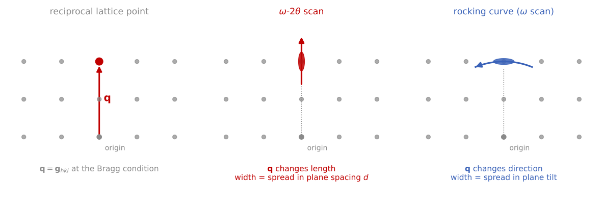
Two scans through one reciprocal lattice point. Left: at the Bragg condition, reaches a reciprocal lattice point. Middle: the - scan moves along its length, through a spot stretched by a spread in plane spacing from strain and composition gradients. Right: the rocking curve swings at constant length, through a spot stretched by a spread in plane tilt from mosaic structure and dislocations.
A reciprocal space map (RSM) scans both and around an asymmetric reflection (one whose planes are inclined to the surface), resolving the in-plane and out-of-plane lattice parameters separately. This is the definitive measurement of coherent strain: a pseudomorphic film appears at the same in-plane reciprocal coordinate as the substrate, while a relaxed film moves toward its bulk lattice constant, and partial relaxation puts it in between, with the relaxed fraction read directly off the map. Around symmetric reflections of thin coherent films, Laue thickness fringes appear: subsidiary maxima spaced by , the diffraction signature of a finite number of coherently scattering planes. Their presence certifies a flat, coherent film and gives its thickness; fitting the full profile with dynamical diffraction theory (which accounts for multiple scattering in thick perfect crystals, where the kinematic single-scattering picture used above breaks down) refines composition and strain in multilayer stacks to high precision.
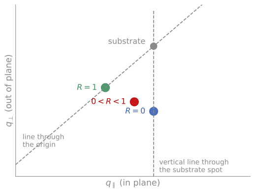
Reading relaxation from a reciprocal space map. A pseudomorphic film () keeps the in-plane lattice parameter of the substrate, so its spot lies directly below the substrate spot. A fully relaxed film () has its bulk lattice parameter in both directions, so its spot lies on the line through the origin and the substrate spot. A partly relaxed film lies between them. Drawn for a film with a larger lattice parameter than the substrate.
Grain size and microstrain
Peak widths measure how far the lattice is coherent. The Scherrer relation,
estimates the coherently diffracting domain size from the peak width (in radians, corrected for instrumental broadening), with the X-ray wavelength, the Bragg angle, and a shape factor. Two cautions apply. Domain size and microstrain both broaden peaks, but with different angle dependence: size broadening goes as while strain broadening goes as , and the Williamson-Hall construction (plotting against ) separates the two, with the intercept giving size and the slope giving microstrain. And the coherent domain is not the grain: subgrain boundaries, stacking faults, and columnar growth all cut coherence, so Scherrer sizes below the film thickness usually signal defected or columnar growth rather than literal grains. Grain-by-grain confirmation belongs to EBSD and TEM.
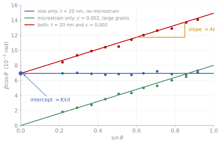
Williamson-Hall plot for three simulated films, with one point per diffraction peak. Blue: 20 nm domains and no microstrain, so every peak has the same and the line is flat. Green: large grains with a microstrain , so the line passes through the origin. Red: both effects together. The intercept gives the domain size , and the slope gives the microstrain.
Texture and stress
Most sputtered and evaporated films are textured: their grains share a preferred out-of-plane orientation while remaining random in-plane (a fiber texture). A pole figure maps the intensity of one reflection over all sample tilts and rotations , revealing fiber textures as rings and epitaxial relationships as discrete spots; quantitative work reduces pole figures to an orientation distribution function. Texture controls properties from electromigration resistance in interconnects to the coercivity of magnetic films, and connects directly to the grain-by-grain orientation maps of EBSD.
Residual stress is measured by using the lattice itself as a strain gauge. In the method, the spacing of one set of planes is measured at several tilts away from the surface normal. For an equi-biaxial film stress , linear elasticity gives a lattice spacing that varies linearly in with slope proportional to , so the stress follows from a straight-line fit and the film’s elastic constants. Thin film stresses routinely reach hundreds of MPa to several GPa, enough to curl substrates, crack coatings, and shift device characteristics; the diffraction measurement complements the wafer-curvature (Stoney) method, which measures the same stress mechanically and needs no crystallinity at all.
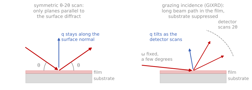
Thin-film XRD geometries. In the symmetric scan, stays pinned to the surface normal, so only planes parallel to the surface diffract. In grazing incidence, the shallow fixed keeps the beam in the film while the detector alone scans.
References and further reading
B. D. Cullity and S. R. Stock, Elements of X-Ray Diffraction, 3rd ed., Prentice Hall (2001). The standard general text; Chapters 1 to 7 cover everything in the first half of this page.
M. Birkholz, Thin Film Analysis by X-Ray Scattering, Wiley-VCH (2006), Chapters 1 to 6. The film-specific methods.
P. F. Fewster, X-Ray Scattering from Semiconductors, 2nd ed., Imperial College Press (2003). High-resolution methods and RSMs.
U. Welzel et al., Stress analysis of polycrystalline thin films and surface regions by X-ray diffraction, Journal of Applied Crystallography 38, 1 (2005). Welzel et al. (2005)
- Welzel, U., Ligot, J., Lamparter, P., Vermeulen, A. C., & Mittemeijer, E. J. (2005). Stress analysis of polycrystalline thin films and surface regions by X-ray diffraction. Journal of Applied Crystallography, 38(1), 1–29. 10.1107/s0021889804029516