

Transmission electron microscopy answers the question every depth-profiling technique in this course approximates: what does the buried interface actually look like? Prepare a cross-section thin enough for electrons to pass through, and the film stack, its interfaces, its defects, and its atomic structure are imaged directly, at resolution down to well below an angstrom. The price is the preparation: the sample must be thinned to below about 100 nm, almost always by FIB lift-out, and the analyzed region is measured in micrometers. This page covers imaging and diffraction in the transmission microscope, emphasizing the scanning (STEM) mode that now dominates materials work; the next page adds spectroscopy.
| At a glance | |
|---|---|
| Probe in / signal out | 60 to 300 keV focused electron beam transmitted through a thin sample |
| Information | Direct imaging of interfaces, layers, and defects down to atomic resolution; local crystal structure and orientation by diffraction |
| Sample thickness | Below about 100 nm; below 30 nm for the highest resolution |
| Lateral resolution | Sub-angstrom probes in aberration-corrected instruments |
| Sensitivity | Single atomic columns; single dopant atoms in favorable cases |
| Sample requirements | Electron-transparent lamella, typically FIB-prepared; preparation is destructive |
Fast electrons and the resolution problem
At 100 to 300 kV, electrons are relativistic and their wavelengths are picometers (about 2.5 pm at 200 kV, computed with the relativistic correction), hundreds of times smaller than an atom. Diffraction therefore never limits TEM resolution; the lenses do. Round magnetic lenses suffer unavoidable spherical aberration (rays through the lens periphery focus too strongly, an aberration Scherzer proved cannot be eliminated in any static round lens) and chromatic aberration (energy spread focuses at different planes). For half a century resolution was set by balancing spherical aberration against diffraction at an optimal aperture, stranding microscopes near 1 to 2 Å. Multipole aberration correctors, standard on high-end instruments since the mid-2000s, cancel the spherical aberration with non-round optics and push probes and images below 0.5 Å, which in practice means every crystalline material resolves into atomic columns when aligned along a low-index axis.
Two operating modes share the column. Conventional TEM illuminates the sample broadly and forms an image with post-specimen lenses; STEM focuses the beam to a fine probe, scans it, and records scattered intensity on detectors below, building the image pixel by pixel exactly as in the SEM. The two are related by reciprocity (a STEM detector plays the role of a TEM source, and vice versa), so their contrast mechanisms mirror each other; STEM’s practical advantages, directly interpretable incoherent contrast and simultaneous multi-signal collection, have made it the default for materials work, and this course follows that usage.
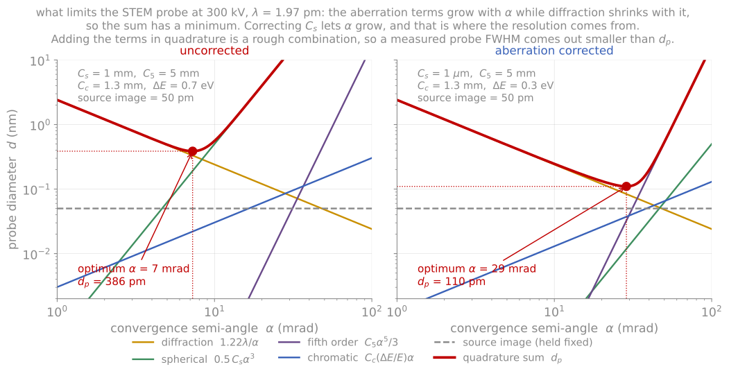
Each contribution to the probe diameter against convergence semi-angle at 300 kV, with the quadrature sum and its optimum, for an uncorrected and an aberration-corrected instrument.
Contrast: what makes an image
The beam leaving a thin sample carries several distinguishable signals, and detector geometry selects among them:
High-angle annular dark field (HAADF) collects electrons scattered to high angles (inner angle several tens of milliradians) by near-nucleus, Rutherford-like scattering. Intensity scales roughly as per atom and increases monotonically with thickness, giving directly interpretable atomic-number contrast: heavy layers bright, light layers dark, without the contrast reversals of phase-contrast imaging. HAADF is the default structural image of a film stack, and the mode meant by “Z-contrast.”
Bright field (BF) collects the transmitted disk. In crystalline samples its contrast at medium resolution is diffraction contrast: any region satisfying a Bragg condition scatters intensity out of the BF detector and appears dark. This is the classical language of defect imaging: bend contours sweep through elastically bent regions, thickness fringes stripe wedge-shaped foils, and strain fields of dislocations light up against background, with the textbook invisibility criterion (a dislocation vanishes when its Burgers vector lies in the reflecting plane, ) still the standard way to identify Burgers vectors.
Annular bright field (ABF), the rim of the transmitted disk, renders light-element columns (oxygen, nitrogen, lithium) visible alongside heavy ones, recovering the light elements that Z-contrast misses.
Pixelated detectors record the full diffraction pattern at every probe position (4D-STEM), from which any of the above contrasts can be synthesized after the fact, and quantities like local strain, orientation, polarity, and electromagnetic field maps can be computed. We keep 4D-STEM to a mention here; its methods are good final-project topics.
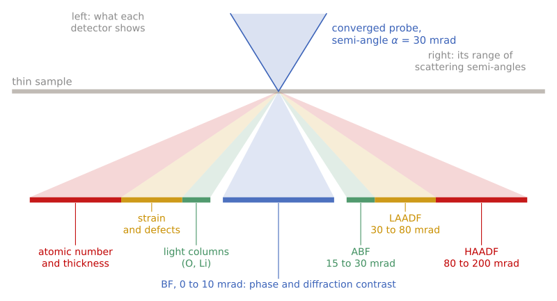
Detector geometry, in side view and not to scale. Each detector is a ring below the sample that collects a range of scattering semi-angles (right labels, for a 30 mrad probe at 300 kV) and shows a different kind of contrast (left labels). Modern instruments record several at once.
Underneath all crystalline-sample imaging sits dynamical diffraction: a fast electron in a crystal does not scatter once but channels and exchanges intensity among beams continuously, with a characteristic length (the extinction distance, tens of nanometers) over which intensity oscillates between the direct and diffracted beams. This is the origin of the thickness fringes above, the reason image intensities are not simply proportional to scattering power, and the reason quantitative comparisons lean on simulation (the multislice method; see the simulation appendix). HAADF’s popularity rests on being the most forgiving of these effects, incoherent enough that simple interpretation usually holds, but honest atomic-scale quantification still checks against simulation.
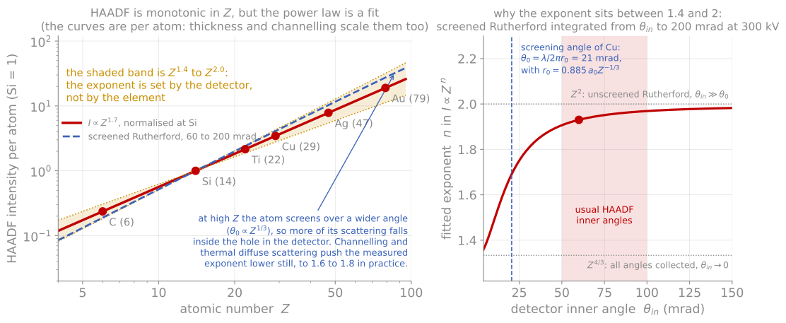
HAADF intensity against atomic number with the line, and the second panel showing how the exponent runs from 4/3 to 2 as the detector inner angle moves out past the screening angle.
Diffraction in the microscope
The same instrument is a diffraction camera with a selectable probe size, and the diffraction modes are organized by convergence angle:
Selected-area electron diffraction (SAED): parallel illumination over a chosen sub-micrometer region gives single-crystal spot patterns that identify phases and orientation relationships across an interface, the local, single-grain complement to the ensemble average of XRD. Indexing a zone-axis pattern (ratios of spot spacings plus interplanar angles) is a core skill inherited directly from the reciprocal-lattice machinery of Module 2.
Convergent-beam electron diffraction (CBED): focusing the beam turns spots into disks whose internal intensity structure encodes specimen thickness and full crystal symmetry (including the point-group information that spot positions alone cannot give).
Nanobeam / scanning electron diffraction: a small-convergence probe scanned across the sample yields a pattern per position; tracking the Bragg disk positions maps local lattice parameters, and hence strain, at a few nanometers resolution with about 10-3 precision, directly on the device feature of interest.
Where the reciprocal-space rods of RHEED and LEED probed the surface, transmission diffraction probes the full foil thickness, and the same Ewald constructions carry over with one addition: the finite foil thickness relaxes the third Laue condition into short rods (rel-rods) along the beam direction, the transmission cousin of the surface-rod physics of the previous page.
Projection
Every TEM and STEM image is a projection through the full thickness of the foil, and forgetting this is the most common way to misread one. A rough interface viewed edge-on projects into an apparently diffuse interface: the measured “interfacial width” is the roughness amplitude folded through the lamella thickness, not the chemistry. An inclined interface does the same, with the apparent width growing linearly with lamella thickness. The only case where the apparent width is the real chemical width is a flat, chemically graded interface, and distinguishing these cases from a single image is not possible. In practice we check by comparing two orthogonal cross-sections, by thinning the lamella further and watching whether the apparent width shrinks, or by tilting.
Projection simulation
The demonstration below makes the geometry explicit for the two standard specimen geometries. A cross-section (the FIB lift-out of the previous page) views the film edge-on: interfaces appear directly, and the projection error is set by the lamella thickness. Plan view (often just the film floated or back-thinned, far easier preparation) views along the film normal: lateral structure appears clearly, but a flat buried interface produces no contrast at all, sharp or diffuse. Run the interface types against both views and note the apparent-width readout: for a rough interface it tracks the lamella thickness, which is why the lamella thickness should be reported alongside any published interface width. The chemical mixing slider broadens the same readout through real interdiffusion, and comparing the two is the exercise: geometric projection and true chemistry produce the same blur in a single image.
Other things to keep straight
Three more items belong on the checklist. The FIB lamella carries amorphized surface layers and implanted Ga on both faces, so the outer few nanometers of the sample are preparation, not material, and the thinner the lamella the larger the corrupted fraction. Beam damage (knock-on displacement at high voltage, radiolysis in insulators and organics) can modify a sensitive sample faster than it can be imaged; the controls are voltage, dose rate, total dose, and cryo. And dynamical diffraction means intensities are not proportional to scattering power, so quantitative claims about atomic-scale intensities need to be checked against simulation.
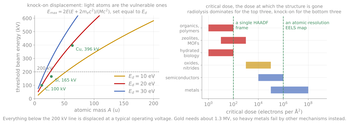
What limits the dose. Knock-on displacement threatens light atoms at the voltages we use, radiolysis threatens insulators and organics, and the critical dose of the material has to be compared against the dose the measurement needs.
References and further reading
D. B. Williams and C. B. Carter, Transmission Electron Microscopy, 2nd ed., Springer (2009). The comprehensive text, including all of diffraction contrast.
S. J. Pennycook and P. D. Nellist (eds.), Scanning Transmission Electron Microscopy: Imaging and Analysis, Springer (2011).
C. Ophus, Quantitative scanning transmission electron microscopy for materials science: imaging, diffraction, spectroscopy, and tomography, Annual Review of Materials Research 53 (2023). Ophus (2023)
- Ophus, C. (2023). Quantitative Scanning Transmission Electron Microscopy for Materials Science: Imaging, Diffraction, Spectroscopy, and Tomography. Annual Review of Materials Research, 53(1), 105–141. 10.1146/annurev-matsci-080921-092646