A 4D-STEM dataset from a complex microstructure can contain thousands of distinct diffraction patterns: different phases, orientations, domains, and overlaps. Designing virtual detectors by hand (as in the previous module) works when you know what you are looking for; unsupervised machine learning lets the data tell you what distinct patterns exist and where they occur, with no prior assumptions about the structures present Martineau et al. (2019).
The idea
Treat each probe position as one observation (a vector of detector-pixel intensities) and ask: what small set of characteristic patterns, mixed in varying proportions, explains the whole dataset? Two families of methods are widely used:
Matrix decomposition (PCA, non-negative matrix factorization): factorize the data into a set of component patterns and their real-space loading maps. NMF’s non-negativity constraint suits diffraction data, since patterns and mixing weights are both inherently non-negative. PCA is often used first for denoising and to estimate how many components the data supports (scree plot).
Clustering: group similar observations, giving a hard segmentation of the field of view into phases/domains, with each cluster’s mean pattern available for crystallographic interpretation. Centroid methods (k-means, Gaussian mixtures) require choosing the number of clusters up front; density-based methods (DBSCAN and its relatives) instead take density threshold parameters and find as many clusters as the data supports arXiv:2606.23201. The observations need not be whole patterns: clustering the detected Bragg peaks themselves in combined real and diffraction space is the basis of the clustering-based digital dark field workflow in this session’s tutorial.
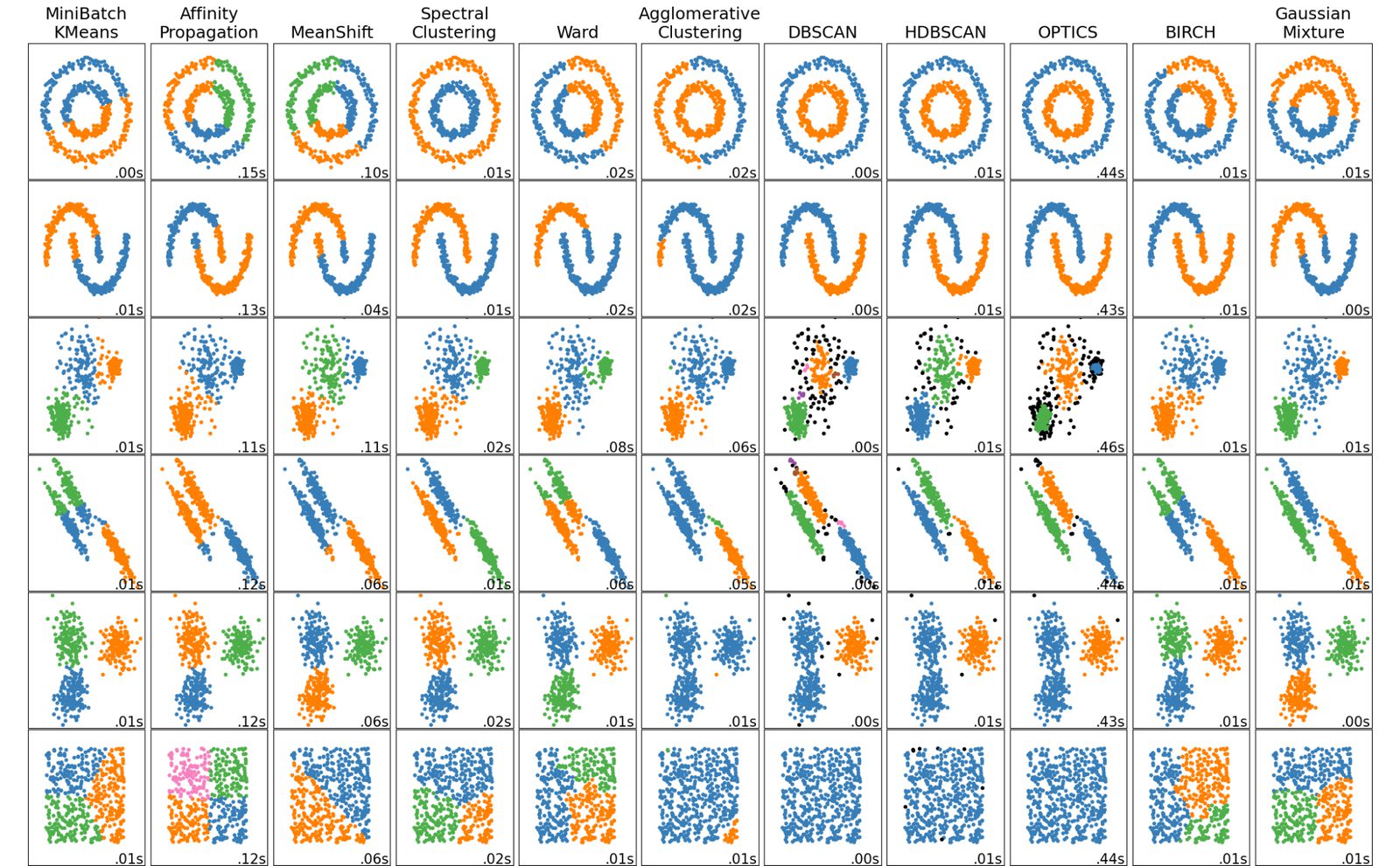
No single “right” clustering algorithm: the scikit-learn comparison grid shows how k-means, spectral, agglomerative, DBSCAN, Gaussian-mixture, and other methods partition the same toy datasets very differently. The same is true for diffraction data.
A typical workflow: preprocess (align the zero beam, mask the central disk or take a log/power scaling so weak reflections count, optionally bin) → reduce dimensionality → decompose or cluster → inspect the component patterns as diffraction patterns and interpret them crystallographically → refine.
Why this works so well for diffraction data
Unlike natural images, diffraction patterns from a given phase/orientation are highly reproducible; the “signal manifold” is low-dimensional. Clustering therefore tends to recover physically meaningful classes: distinct phases, orientation variants, ordered vs. disordered regions, and even subtle symmetry-breaking distortions that are hard to see by eye Kalinin et al. (2022). The output is a phase/domain map plus a library of representative patterns, obtained in minutes from datasets far too large to inspect manually:
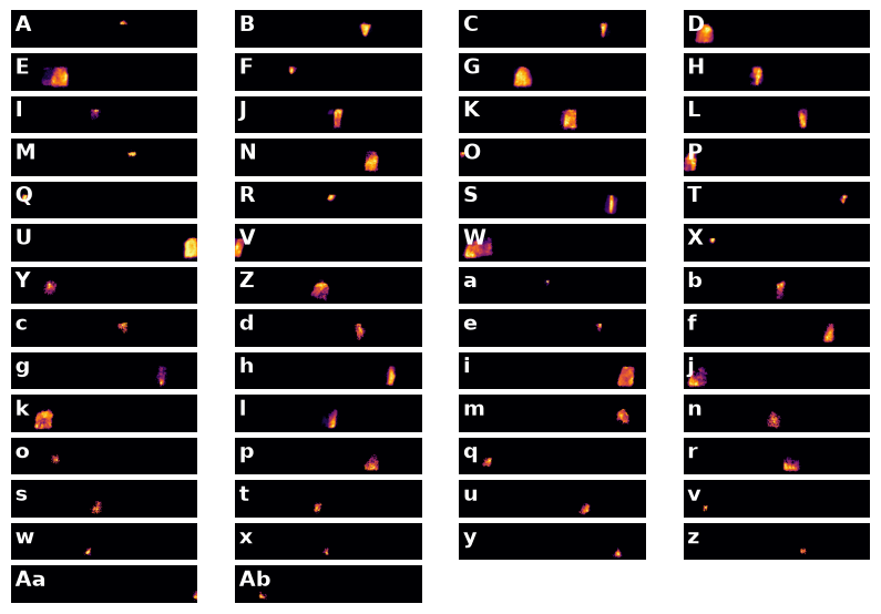
The payoff: each cluster’s mean diffraction pattern, extracted automatically from a 4D-STEM scan. Each class corresponds to a distinct diffraction condition (a phase, orientation variant, or overlap), ready for crystallographic interpretation.
Caveats
Components are mathematical objects, not guaranteed physics: decomposition can mix or split physical phases (e.g., NMF components need not correspond one-to-one with real structures). Always validate components against the raw patterns and against crystallographic simulation.
Intensity scaling choices (log, power, masking the direct beam) strongly affect what the algorithms consider “similar”; dynamical intensity variations within one grain can otherwise dominate over phase differences.
Density-based clustering does not assign every point, and that is fine. The unclustered leftovers include very small diffracting objects, false detections, and poor detections shifted well off the true disk centroid. The density parameters set the smallest object you wish to see (e.g.
min_samples = 20), and even without analysing every disk you get far more clusters than you would ever analyse manually.
- Martineau, B. H., Johnstone, D. N., van Helvoort, A. T. J., Midgley, P. A., & Eggeman, A. S. (2019). Unsupervised machine learning applied to scanning precession electron diffraction data. Advanced Structural and Chemical Imaging, 5(1). 10.1186/s40679-019-0063-3
- Kalinin, S. V., Ophus, C., Voyles, P. M., Erni, R., Kepaptsoglou, D., Grillo, V., Lupini, A. R., Oxley, M. P., Schwenker, E., Chan, M. K. Y., Etheridge, J., Li, X., Han, G. G. D., Ziatdinov, M., Shibata, N., & Pennycook, S. J. (2022). Machine learning in scanning transmission electron microscopy. Nature Reviews Methods Primers, 2(1). 10.1038/s43586-022-00095-w