

This page completes the electron spectroscopy module with the working skills: converting XPS peak areas into compositions and layer thicknesses, Auger electron spectroscopy as the focused-probe counterpart to XPS, and the sputter depth profiling that turns both into layer-by-layer analysis.
Quantifying XPS
The intensity of a photoelectron line from a homogeneous sample is proportional to the atomic concentration times a chain of instrument and physics factors: the photoionization cross section of the level, its angular emission asymmetry, the IMFP at that kinetic energy, and the analyzer transmission at that energy. In practice the chain is collapsed into empirical relative sensitivity factors (either Scofield-cross-section-based with instrument corrections, or fully empirical sets measured on standards), and compositions follow from
Here is the atomic fraction of element , is its measured peak area, is its sensitivity factor, and the sum runs over every element detected. The peak areas must first be separated from the inelastic background, and the choice of background matters at the few-percent level: the pragmatic standard is the Shirley background, which grows in proportion to the integrated peak above it; the physically grounded alternative is the Tougaard method, which models the actual inelastic scattering. Done carefully, XPS composition is accurate to 5 to 10% relative, with two standing caveats. The answer is an exponentially weighted average over the sampling depth, so any vertical inhomogeneity (a contamination layer, an oxide skin, segregation) biases it, and the direction of the bias follows directly from the weighting: whatever is on top is overcounted. And adventitious carbon sits on every sample that has seen air, attenuating everything beneath it.
The same escape-depth physics measures overlayer thickness, one of the most-used quantitative results in surface analysis. For a uniform overlayer of thickness on a substrate, the substrate line is attenuated by while the overlayer line grows with the complementary factor ; ratioing the two cancels the X-ray flux and most instrument factors, and inverting gives directly for films up to about . This ratio method, and its angle-resolved extension in which spectra at several emission angles are inverted into a depth profile of the top few nanometers, is the workhorse measurement of gate oxides, ALD nucleation, self-assembled monolayers, and surface cleans: nondestructive, standardless, and accurate to a few percent for films under about 10 nm, provided the IMFP values and the assumed layer model (uniform, continuous) are accurate. Island growth misread as a thin uniform layer is the classic failure, and checking the angle dependence is how it is caught.
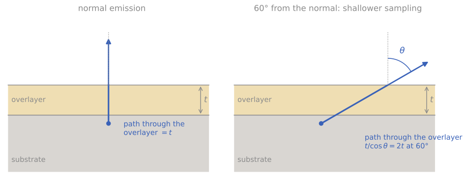
Why tilting makes XPS more surface sensitive. A photoelectron from the substrate (blue) crosses an overlayer of thickness . At normal emission its path through the overlayer is ; at 60° from the normal it is , so the substrate signal is attenuated more and the overlayer signal is relatively stronger.
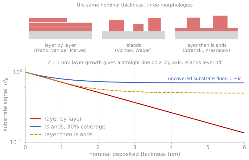
The same nominal thickness in three morphologies, and the substrate signal each one produces. Layer growth gives a straight line on a log axis; islands level off at the uncovered fraction.
Auger electron spectroscopy
When a core hole is filled, the released energy can eject a second electron instead of an X-ray: the Auger process, a three-level transition labeled by the shells involved (KLL, LMM, MNN, ...). Its kinetic energy is approximately the core-level energy minus the binding energies of the two outer participants (with a correction for the doubly ionized final state), a property of the atom alone, independent of how the initial hole was made and of the excitation energy. Auger electrons therefore appear in every XPS spectrum; Auger electron spectroscopy (AES) as a standalone technique excites them with an electron beam instead of X-rays, and that one change defines its niche. An electron beam focuses to nanometers, so AES delivers surface chemical analysis with lateral resolution some three orders of magnitude better than laboratory XPS: about 10 nm in a modern field-emission scanning Auger microprobe, with secondary-electron imaging built in to find the feature of interest.
The fluorescence-yield branching makes the Auger channel dominant for light elements, exactly where EDS is weakest, and the detected electrons obey the same escape-depth physics as XPS, sampling a few nanometers. Because the Auger peaks ride on the large, sloping secondary-electron background, spectra were historically recorded in derivative mode, , and much of the literature and the standard sensitivity-factor sets are built on derivative peak-to-peak heights; modern instruments record direct spectra and integrate. Quantification with sensitivity factors is semiquantitative (10 to 20%) unless matrix-matched standards are used; chemical-state information exists (the carbon KLL lineshape famously distinguishes carbide, graphite, and diamond) but is less systematic than XPS shifts. The electron beam also brings limitations: charging restricts AES to reasonably conductive samples far more strictly than XPS, and the focused beam’s current density can damage or modify sensitive surfaces during the measurement.
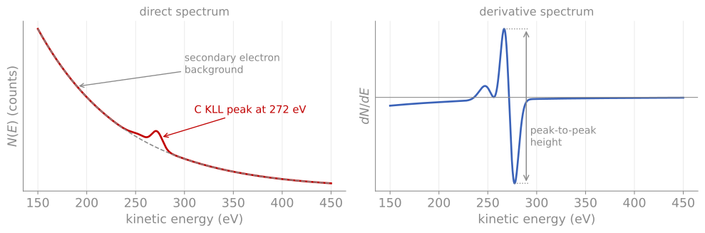
Direct and derivative Auger spectra. Left: the C KLL Auger peak at 272 eV on the secondary-electron background (dashed). Right: the same spectrum differentiated, which suppresses the slowly varying background; the peak-to-peak height is the signal used by the classic sensitivity-factor tables.
The applications that exploit these strengths involve identifying small features: particle and defect identification on wafers (the historical backbone of semiconductor failure analysis), grain-boundary chemistry on fracture surfaces exposed in situ (the classic measurements of temper embrittlement, where segregated phosphorus monolayers at boundaries were measured directly), and small-area depth profiles of metallization stacks.
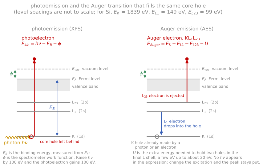
Why the Auger lines move when you change the anode and the photoelectron lines do not: the photoelectron energy carries and the Auger energy does not.
Sputter depth profiling
Both XPS and AES sample only a few nanometers; to profile deeper, both are combined with the sputtering of an argon ion gun, alternating erosion and measurement to build composition versus depth through films hundreds of nanometers thick. Everything learned about sputtering applies as limitations here, and the measured profile is the true profile convolved with a resolution function whose three physical contributions are worth keeping separate: atomic mixing by the ion cascade (pushes species inward, producing exponential trailing edges), surface roughening that accumulates with sputtered depth, and the information depth of the spectroscopy itself (a few ). Depth resolution of a few nanometers is standard; it improves with lower ion energy and grazing ion incidence (thinner mixing layer), with sample rotation during sputtering (suppresses roughening), and with cluster ion sources, whose gentler, shallower impacts profile polymers and organic films with minimal chemical damage. Preferential sputtering adds a chemistry artifact on top of the geometry: compounds whose components sputter unequally develop altered surface compositions, and reducible oxides are famously reduced by ion bombardment, so a “metallic” component appearing during a profile of an oxide must be interpreted with suspicion.
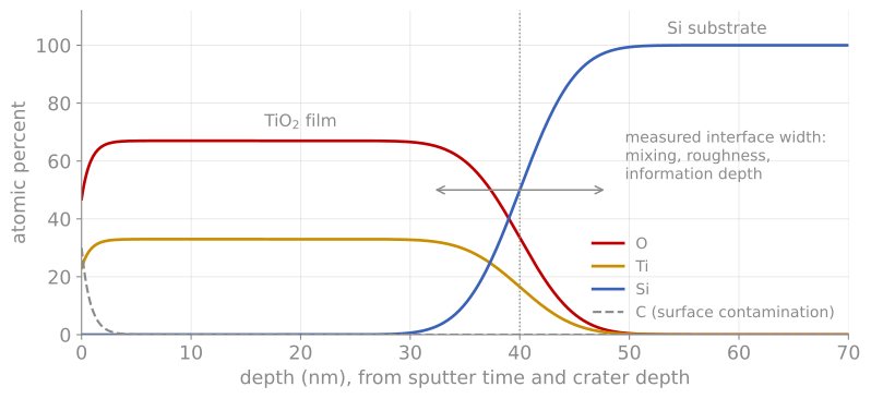
A sputter depth profile. XPS composition against depth for a 40 nm TiO film on Si (schematic). The adventitious carbon disappears in the first nanometer of sputtering, and the interface appears several nanometers wide even though the real interface is sharp, the combined effect of mixing, roughening, and the information depth.
Interpreting any sputter profile means holding the measured curve and the artifact list in mind at once: a measured interface width is an upper bound, not a measurement, unless the sputtering conditions have been qualified on a known sharp interface. When the depth scale must be trusted, the crater is measured afterward with a profilometer; when the interface itself is the science, the nondestructive routes (angle-resolved XPS, MEIS, XRR) or direct STEM cross-sections are the cross-checks.
Choosing among the depth-profiling methods now available: XPS profiling for chemistry versus depth, SIMS for trace sensitivity, angle-resolved XPS or MEIS for nondestructive ultra-shallow profiles, and STEM cross-sections when direct imaging of the actual interface is worth the sample preparation.
References and further reading
D. Briggs and M. P. Seah (eds.), Practical Surface Analysis, Vol. 1, 2nd ed., Wiley (1990). The standard practitioner’s reference for everything on this page.
J. F. Watts and J. Wolstenholme, An Introduction to Surface Analysis by XPS and AES, 2nd ed., Wiley (2020), Chapters 3 to 5.
S. Hofmann, Auger- and X-Ray Photoelectron Spectroscopy in Materials Science, Springer (2013). Includes the quantitative treatment of depth-profile resolution functions.