
Atom probe tomography (APT) is the logical endpoint of the mass spectrometry idea: remove the atoms of a sample one at a time, identify each one by time-of-flight mass spectrometry, and record where each came from. The result is a three-dimensional reconstruction containing tens to hundreds of millions of atoms, each with elemental (and isotopic) identity and a position good to a fraction of a nanometer. No other technique measures the three-dimensional chemistry of a buried interface, a grain boundary, or a dopant cluster with anything approaching this combination of spatial resolution and ppm-level sensitivity, and APT has moved in two decades from a specialist’s curiosity to a mainstream tool of thin film and interface science.
| At a glance | |
|---|---|
| Probe in / signal out | High field plus voltage or laser pulses in; field-evaporated ions out to a position-sensitive ToF detector |
| Information | 3D composition maps with near-atomic resolution; all elements including H and Li, with isotopes |
| Analyzed volume | Roughly 100 nm diameter by up to a micrometer deep |
| Spatial resolution | About 0.1 to 0.3 nm in depth, somewhat coarser laterally |
| Sensitivity | Tens of ppm, uniform across the periodic table |
| Sample requirements | A needle-shaped specimen of about 100 nm tip radius, prepared by FIB; fully destructive |
Field evaporation
Electric fields at surfaces are amplified by curvature: a voltage applied to a needle of apex radius produces an apex field of order with a geometry factor, so 5 to 10 kV on a 50 to 100 nm tip reaches fields of tens of volts per nanometer, the scale required to ionize surface atoms. At such fields, a surface atom can be removed as an ion: the field tilts the energy landscape until the barrier separating the bound atom from the ionic state (in the classical picture, the maximum of the atom’s image-charge potential) falls to the order of thermal energies, and the atom escapes, a process called field evaporation. Because the escape is thermally activated over a field-lowered barrier, evaporation rate depends extremely steeply on field, which is what makes controlled, one-atom-at-a-time removal possible: the specimen is held just below threshold and a small perturbation triggers evaporation preferentially at the most protruding, highest-field atoms, so the tip disassembles in an orderly way from its apex. Each element has its own evaporation field (roughly 10 to 60 V/nm across the periodic table), a fact that returns below as an artifact. Holding the tip below that threshold, rather than at it, is what makes the section that follows possible.
The perturbation that triggers evaporation is the pulse, and its two forms define the instrument families. Voltage pulsing adds a nanosecond high-voltage pulse to the standing voltage; it gives the sharpest timing but requires a conductive specimen to transmit the pulse. Laser pulsing focuses picosecond laser pulses onto the apex, whose brief thermal excitation triggers evaporation at the standing field; it works for semiconductors and insulators, which is what opened APT to microelectronics, oxides, and geology, essentially all thin film work. The cost of laser pulsing is thermal: the tip must cool between pulses, and slow cooling smears evaporation times and hence the mass spectrum. Specimens are held at cryogenic temperature (tens of kelvin) throughout, both to suppress surface diffusion that would scramble positions and to keep the thermally activated evaporation under the pulse’s control.
Field ion microscopy
Field ion microscopy (FIM) is the ancestor of the atom probe and still the way an atom probe specimen is inspected before it is consumed. Erwin Müller built the first one in 1951, and by 1955 it was resolving individual atoms on a tungsten surface, the first images of single atoms ever made. It uses the same needle as APT and the same field amplification by curvature, but instead of removing the surface atoms it uses them to ionize a gas.
The chamber is backfilled with an inert imaging gas, helium or neon, at about 10-5 Torr, and the specimen is held at 20 to 80 K and at a positive voltage below the evaporation threshold. Gas atoms are polarized by the field gradient and pulled toward the apex, where they lose energy by hopping across the cold surface until they are thermally accommodated. A gas atom sitting about 0.4 nm above a surface atom is then field ionized: the field tilts the vacuum level so far that an electron tunnels from the gas atom into an empty state in the metal above the Fermi level, and the resulting positive ion is repelled radially outward to a detector or phosphor screen. Ionization is exponentially sensitive to field, so it happens almost entirely over the atoms that protrude furthest, which are the atoms at the edges of the terraces.
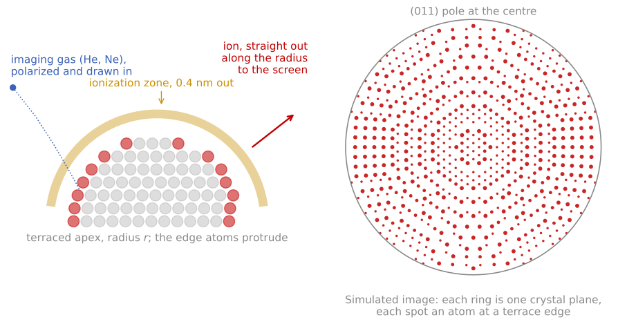
Left: the imaging gas is drawn to the apex, ionizes in a thin zone about 0.4 nm above the atoms that protrude at the terrace edges, and the ion leaves along the radius. Right: a simulated image of a bcc tungsten tip along (011), with each atom placed by projecting the terrace-edge atoms of a hemispherical crystal. Each ring is one crystal plane.
The field needed to ionize the gas is a property of the gas, called the best image field: about 44 V/nm for helium, 35 V/nm for neon, and 22 V/nm for hydrogen. Helium gives the highest resolution because it requires the highest field and so ionizes in the smallest volume, but the field it needs also puts the largest mechanical stress on the specimen. The electrostatic tensile stress at a surface carrying a field is
with the stress in Pa, the vacuum permittivity, and the field in V/m, which is 8.6 GPa at the helium imaging field and 5.4 GPa at the neon field. That number is why classical FIM was done on tungsten, iridium, rhenium, and other refractory metals: anything weaker is pulled apart before it images. Choosing neon, or hydrogen at 2.1 GPa, trades resolution for a specimen that survives.
The image is a radial projection of the apex, magnified by the ratio of the flight distance to the tip radius,
where is the magnification, is the tip-to-screen distance of 50 to 100 mm, is the apex radius of 10 to 100 nm, and is the image compression factor, which accounts for the trajectories being less divergent than a true point projection because the tip is a shank and not an isolated sphere. A 50 nm tip at 60 mm therefore images at about times, with a resolution of 0.2 to 0.3 nm set by the size of the ionization zone and by the tangential velocity the gas atom retains, which is why the specimen is cold.
What the image shows follows from which atoms ionize. A crystal truncated by a roughly hemispherical surface exposes a set of terraces, and only the atoms at the terrace edges protrude enough to image, so each crystallographic plane appears as a ring of bright spots and each pole as the centre of a set of concentric rings. The ring pattern is a map of the crystallography of the tip, which is how the orientation of an atom probe specimen is determined before a run, and counting rings as they disappear during field evaporation counts the planes removed, which is the most direct depth calibration in the technique.
FIM images point defects directly, as a missing or extra spot in an otherwise regular ring, and this is what made it the tool for the early studies of vacancies, of grain boundaries in ordered alloys, and of adsorbed atoms. Surface diffusion measurements made this way are the origin of the Ehrlich-Schwoebel barrier introduced in the properties of surfaces: Ehrlich and Hudda watched single tungsten adatoms hop on a FIM tip, imaging the same atom before and after a controlled anneal, and found that atoms approaching a descending step were reflected rather than crossing it.
Its limits are the ones the method implies. The specimen must be a needle that survives several GPa of tensile stress, the field selects what is imaged so protruding atoms are over-represented and flat low-index terraces appear almost empty, the imaging gas restricts the accessible fields, and the technique gives crystallography and defect structure but no chemical identity. Adding a mass spectrometer behind a probe hole in the screen supplies exactly that missing identity, which is what Müller did in 1968 and what became the atom probe.
The measurement
A modern local-electrode atom probe places a counter-electrode aperture close to the tip, lowering the required voltage and increasing the field of view; ions accelerate through the aperture and fly tens of centimeters to a microchannel-plate detector backed by crossed delay lines that record each impact’s position and time. Two measurements result per ion. The flight time gives the mass-to-charge ratio from the energy balance ; ions arrive in charge states of 1+ to 3+, so the spectrum is indexed in and one element appears at several positions. The impact position, together with the arrival order, encodes the atom’s origin on the tip: the near-hemispherical apex acts as a point-projection microscope with magnification of order 106, set by the flight length over the tip radius times an image-compression factor.
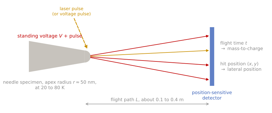
Atom probe layout, not to scale. A needle specimen at a standing voltage loses one surface atom as an ion on each laser or voltage pulse. The ions fly a path to a position-sensitive detector, which records the flight time, giving the mass-to-charge ratio, and the hit position, giving the lateral position on the specimen.
Reading the mass spectrum is a skill of its own. Isotope patterns confirm assignments; hydride adducts (from residual hydrogen), molecular ions, and multiple-hit events complicate them; and some overlaps are genuinely degenerate at the achievable resolution, so composition accuracy varies element pair by element pair. Detection efficiency, set mainly by the open area of the microchannel plates, is roughly 50 to 80% depending on instrument generation: APT counts a known fraction of all atoms, uniformly enough across elements that compositions are reliable, but it never sees every atom.
Reconstruction and its artifacts
Turning the detector record into a 3D atom map is a modeling step, not a direct measurement. The standard protocol inverts the point projection: each ion’s detector position maps back to an apex position through the assumed tip shape, the depth increment advances in proportion to the volume evaporated (each detected atom accounts for its atomic volume divided by the detection efficiency), and the tip radius is evolved as the needle blunts into its taper. Depth resolution is the technique’s greatest strength: because atoms leave layer by layer, atomic planes are routinely resolved along the analysis direction. Lateral resolution is coarser, a few tenths of a nanometer at best, blurred by the trajectory of each ion launching from an atomically rough surface.
Each assumption produces its own artifacts, and quantitative APT requires knowing them. Real multilayer specimens violate the single-radius assumption: phases with different evaporation fields develop different local curvatures, producing local magnification distortions in which low-field phases appear artificially dense (or dilute) and interfaces appear curled; trajectory aberrations concentrate near phase boundaries, which are usually the regions of interest. Species with low evaporation fields can also desorb between pulses (DC evaporation), arriving without a timestamp and being lost preferentially, one mechanism by which detection can become composition-biased. Detector dead time undercounts multiple simultaneous evaporation events, which biases the stoichiometry of compounds that evaporate correlated bursts. None of this diminishes the technique; it defines the error bars, and the community’s standard analyses (composition profiles across interfaces, isoconcentration surfaces with proximity histograms, cluster-finding statistics tested against randomized data) are designed to extract conclusions robust to them.
Field evaporation simulation
The animation below runs the whole idea. The needle contains a multilayer (gold-colored heavy solute bands in a purple matrix) plus one solute cluster. Field evaporation removes atoms from the apex, the evaporation front recedes and widens into the shank, and each detected atom is placed into the reconstruction on the right. Watch what survives and what degrades: the layers and the cluster stay sharp in depth, because depth comes from arrival order; lateral positions blur by a few atom spacings from trajectory aberrations; and the missing atoms bias the measurement, since the matrix is lost more often than the solute and the measured composition shifts accordingly. Compare the true and measured solute fractions in the panel as the run proceeds.
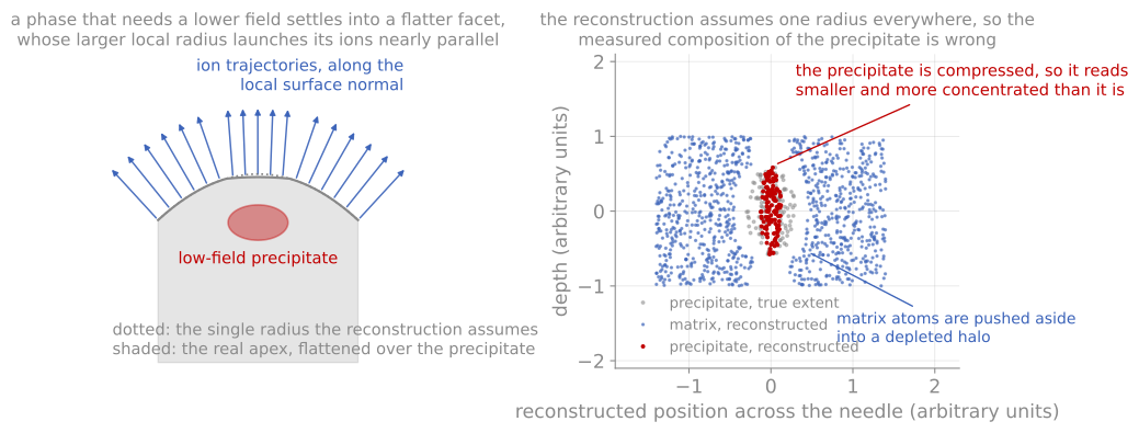
Local magnification. A phase that evaporates at a lower field settles into a flatter facet, its ions leave nearly parallel, and the reconstruction compresses it into something smaller and denser than the real precipitate.
Strengths and limits
The measurements no other technique makes are three-dimensional and chemical at once: the segregation of dopants to a single grain boundary measured in atoms per unit area (the Gibbsian interfacial excess, measured directly by counting), the earliest stages of clustering and precipitation in an alloy, the true interfacial width and intermixing of a deposited multilayer, and the distribution of hydrogen or lithium, light elements invisible to most electron and X-ray spectroscopies, in battery electrodes and embrittled alloys. In semiconductor work it is the only measurement of the 3D dopant distribution in a single finFET fin. Because analysis requires a FIB-milled needle from a specific site, APT pairs naturally with FIB sample preparation, and correlative workflows that image the same needle in STEM before running it in the atom probe tie the reconstruction to crystallography and calibrate its shape assumptions.
The counterweights: throughput is low (hours per needle, and needles fracture under the field stress, more often the harder the material), the analyzed volume is minuscule so statistics demand multiple tips, and quantification near interfaces carries the reconstruction caveats above. APT complements rather than replaces SIMS: SIMS profiles a millimeter-scale area with ppb sensitivity in one dimension, APT maps a hundred-nanometer volume with ppm sensitivity in three.
References and further reading
B. Gault et al., Atom probe tomography, Nature Reviews Methods Primers 1, 51 (2021). Gault et al. (2021)
B. Gault, M. P. Moody, J. M. Cairney, and S. P. Ringer, Atom Probe Microscopy, Springer (2012).
T. F. Kelly and M. K. Miller, Atom probe tomography, Review of Scientific Instruments 78, 031101 (2007). Kelly & Miller (2007)
- Gault, B., Chiaramonti, A., Cojocaru-Mirédin, O., Stender, P., Dubosq, R., Freysoldt, C., Makineni, S. K., Li, T., Moody, M., & Cairney, J. M. (2021). Atom probe tomography. Nature Reviews Methods Primers, 1(1). 10.1038/s43586-021-00047-w
- Kelly, T. F., & Miller, M. K. (2007). Atom probe tomography. Review of Scientific Instruments, 78(3). 10.1063/1.2709758