Ion-Solid Interactions

The next four pages cover techniques that fire ions at a sample: Rutherford backscattering, elastic recoil detection, low-energy ion scattering, secondary ion mass spectrometry, and atom probe tomography. All of them rest on the same physics, developed here: the kinematics of binary collisions, the cross section for scattering, and the stopping of ions as they travel through matter. This physics is worth learning carefully, both because it makes every ion beam technique quantitative from first principles, a property almost unique among the methods in this course, and because the same collisions govern ion implantation, sputter deposition, focused ion beam machining, and radiation damage.

Why the problem is simple¶

Before the formulas, it is worth seeing why ion-solid scattering reduces to classical billiards, because each simplification is an estimate you can check.

No diffraction. The de Broglie wavelength of even a slow ion is tiny: $\lambda = h/\sqrt{2ME}$ gives well below a picometer for a keV noble-gas ion, orders of magnitude smaller than interatomic spacings, so ions travel as classical particles. Contrast the electrons of Module 6, whose wavelengths at low energy match atomic spacings and diffract strongly.
The lattice is frozen. A collision lasts of order 10^-14 s, while lattice vibration periods are of order 10^-12 s: the target atom does not move meaningfully during the collision, so it can be treated as stationary and free.
Chemistry is irrelevant. Bond energies are a few eV; the projectile carries thousands to millions of eV. Binding contributes nothing to the collision itself (though it returns as the surface binding energy in sputtering). Ion scattering therefore measures mass and position, never chemical state, which is XPS territory.
Collisions are binary. Equating the beam energy to the Coulomb energy gives the distance of closest approach $d_c = Z_1 Z_2 e^2 / (4\pi\varepsilon_0 E)$ . For 2 MeV He on silver, $d_c \approx 7 \times 10^{-5}$ nm, far inside the electron cloud and thousands of times smaller than the interatomic spacing: an ion is only ever “close” to one atom at a time, and at these distances the interaction is the bare nuclear Coulomb repulsion. At keV energies $d_c$ grows to the order of the Bohr radius, still well below atomic spacings (collisions stay binary) but now inside a screening cloud of electrons, which is why the screened potentials below take over.

The same estimate of $d_c$ organizes the ion-beam techniques by energy, because the energy sets both the physics and the probing depth:

Beam energy	Technique	Depth probed	Typical use
0.1 to 10 keV	LEIS, SIMS, sputtering, FIB	outermost layers	surface composition, depth profiling, machining
10 to 500 keV	MEIS, implantation	about 10 nm to 1 um	ultra-shallow profiles, doping
0.5 to 5 MeV	RBS, ERD	about 1 um	absolute composition vs depth

Kinematics of elastic collisions¶

Consider a projectile of mass $M_1$ and energy $E_0$ striking a stationary target atom of mass $M_2$ . The collision is simplest in the center-of-mass frame, where the two particles approach with equal and opposite momenta and simply rotate their momenta through the scattering angle $\theta_c$ ; transforming back to the laboratory frame and applying conservation of energy and momentum, with no knowledge of the interaction force whatsoever, fixes the energy of the projectile scattered to laboratory angle $\theta$ :

E_1 = K E_0, \qquad K = \left[ \frac{M_1 \cos\theta + \sqrt{M_2^2 - M_1^2 \sin^2\theta}}{M_1 + M_2} \right]^2 .

(1)

Here $E_0$ is the incident energy, $E_1$ the energy of the projectile after scattering, $M_1$ the projectile mass, $M_2$ the mass of the target atom, and $\theta$ the scattering angle in the laboratory frame. The kinematic factor $K$ depends only on the mass ratio and the scattering angle. This is the central result of the module: measure the energy of a backscattered ion of known mass and energy, and you have measured the mass of the atom it hit. Its limiting behaviors are worth internalizing. Heavy targets barely recoil, so $K \to 1$ and heavy elements crowd together near the beam energy, which is why RBS mass resolution degrades for heavy elements. For $M_2 < M_1$ the square root goes imaginary beyond a maximum angle: backscattering is kinematically forbidden, a light target cannot turn a heavy projectile around, which is why helium beams cannot backscatter from hydrogen and why detecting hydrogen requires the forward-recoil geometry of ERD. At exactly $\theta = 90°$ and $M_1 = M_2$ , $K = 0$ : equal masses exchange all energy, billiard-ball style.

The struck atom recoils at angle $\phi$ (forward of 90° always) with energy

E_2 = \frac{4 M_1 M_2}{(M_1 + M_2)^2} E_0 \cos^2\phi ,

(2)

where $E_2$ is the recoil energy and $\phi$ the recoil angle measured from the beam direction. The transfer reaches the full $4M_1M_2/(M_1+M_2)^2$ fraction in a head-on collision, which for comparable masses approaches complete energy transfer. These energetic recoils drive the collision cascades responsible for sputtering, treated with SIMS, and for implantation damage below.

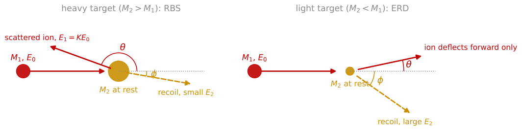
Binary collision of a projectile with a heavier and with a lighter target atom — **One collision, two cases.** A projectile of mass $M_1$ and energy $E_0$ (red) strikes a target atom of mass $M_2$ at rest (gold). A heavier target (left) can send the projectile backward through the scattering angle $\theta$ , keeping $KE_0$ , and recoils with little energy. A lighter target (right) only deflects the projectile forward, and the recoil, leaving at angle $\phi$ , carries much of the energy, which is the geometry of ERD.

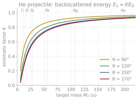
Kinematic factor versus target mass for a helium projectile at four scattering angles — **The kinematic factor.** Computed for a He projectile. The steep region at low mass gives ion scattering its excellent light-element mass resolution; the flattening toward heavy masses is why W and Ta are indistinguishable. Larger scattering angles separate the masses best, which is why detectors sit as far backward as geometry allows.

The scattering cross section¶

How often collisions happen, and how hard they are, is set by the force between the nuclei. For a bare Coulomb repulsion, the classical orbit calculation relates impact parameter to deflection angle and yields Rutherford’s differential cross section, which in the center-of-mass frame is

\frac{d\sigma}{d\Omega} = \left( \frac{Z_1 Z_2 e^2}{4 E} \right)^2 \frac{1}{\sin^4(\theta_c/2)} .

(3)

Here $d\sigma/d\Omega$ is the cross section for scattering into unit solid angle, $Z_1$ and $Z_2$ are the atomic numbers of the ion and the target atom, $e$ is the elementary charge, $E$ is the ion energy, and $\theta_c$ is the scattering angle in the center-of-mass frame. Three scalings matter for analysis. The cross section grows as $(Z_1 Z_2)^2$ , so heavy elements scatter far more strongly than light ones; it falls as $1/E^2$ , so count rates drop quickly with beam energy; and it is known absolutely, with no adjustable parameters, which is what makes RBS a standards-free quantitative technique. The steep $\sin^{-4}(\theta_c/2)$ dependence means small-angle collisions vastly outnumber large-angle ones: an ion in a solid undergoes many small deflections punctuated by rare hard collisions, exactly the structure visible in the trajectories of the simulator below.

The bare-Coulomb result holds only when the collision is close enough that the nuclei see each other’s unscreened charge. At larger distances the atomic electrons screen the interaction, described by multiplying the Coulomb potential by a screening function $\Phi(r/a)$ that falls from one to zero over a screening length $a$ of order 0.1 to 0.5 Å. The modern standard is the ZBL universal potential of Ziegler, Biersack, and Littmark, a four-exponential fit to calculated interatomic potentials that works for essentially any ion-atom pair. The practical division of labor: at MeV energies and large angles (RBS conditions) the collision penetrates the screening and Rutherford holds to within small corrections; at keV energies (LEIS, sputtering, implantation, FIB) screening controls everything, and the scattering must be computed from the screened potential, which is precisely what the simulator on this page does numerically.

Stopping power¶

Between the rare large-angle collisions, an ion moving through a solid loses energy continuously. Two mechanisms operate, and their competition organizes the entire field:

Nuclear stopping: energy transferred to target nuclei in many small screened collisions. It dominates at low velocity, deflects trajectories, and displaces atoms, creating damage. Expressed in the dimensionless reduced units of Lindhard, nuclear stopping is a single universal curve for all ion-target pairs, peaking when the ion velocity is well below the orbital velocities of the target electrons: in practical terms, keV energies for heavy ions.
Electronic stopping: drag from exciting and ionizing target electrons. It behaves differently in two velocity regimes. At low velocity (below the Fermi velocity of the target electrons), the drag is proportional to velocity, $S_e \propto \sqrt{E}$ , the Lindhard-Scharff regime, like viscous friction. At high velocity the Bethe theory applies: stopping falls as $1/E$ times a logarithm, because a fast ion spends less time near each electron. Between them the stopping passes through a maximum (the Bragg peak, near 0.7 MeV for He in most targets), the feature exploited in ion cancer therapy and the reason MeV He ions deposit most of their energy deep in a sample rather than at the surface.

The total stopping power $dE/dx$ is tabulated to few-percent accuracy for essentially all ion-target combinations; the SRIM package, discussed in the simulation appendix, is the community standard, and for a compound target the stopping contributions add in proportion to composition (Bragg’s rule). A 2 MeV He ion in silicon loses roughly 240 eV per nanometer, almost all electronically, and this steady, predictable loss is what converts a measured energy into a depth in RBS and the other ion beam methods. A useful unit habit: because films are better characterized by atoms per area than by thickness, stopping is often quoted as a stopping cross section $\varepsilon = (dE/dx)/n$ in eV·cm $^2$ /10 $^{15}$ atoms, which removes the density from the bookkeeping.

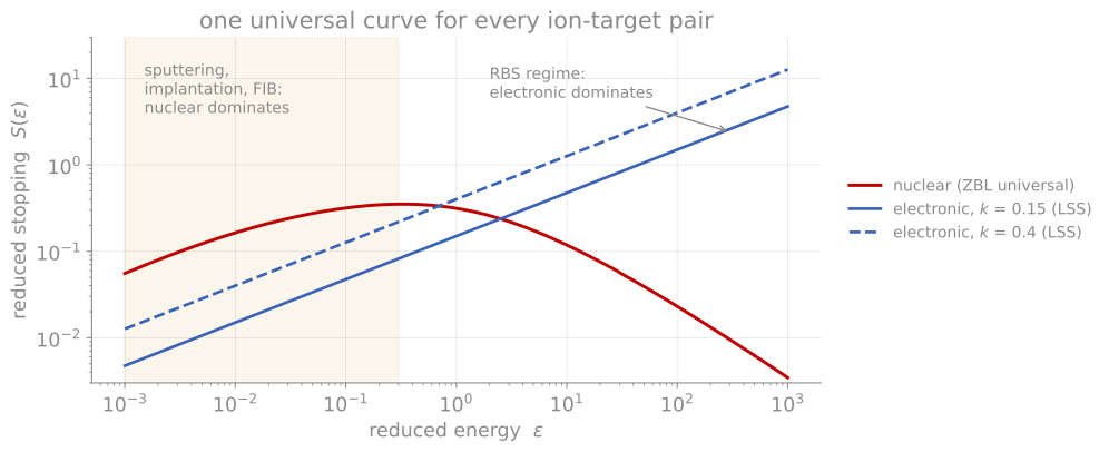
Universal reduced nuclear stopping curve and velocity-proportional electronic stopping lines versus reduced energy — **Universal stopping curves.** Stopping in Lindhard’s reduced units, where one nuclear-stopping curve serves every ion-target pair. Nuclear stopping dominates at low reduced energy (the sputtering and implantation regime) and electronic stopping, rising as the square root of energy, dominates at high reduced energy (the RBS regime).

Range, straggling, and damage¶

Stopping ends in a range. Ions implanted at energy $E_0$ come to rest in a roughly Gaussian depth distribution with projected range $R_p$ and straggle $\Delta R_p$ , from a few nanometers at keV energies to micrometers at MeV energies. The statistics matter as much as the mean: straggling arises because each ion’s sequence of collisions is random, and light ions in heavy targets also backscatter out entirely. Skewness appears when nuclear stopping dominates (heavy slow ions pile up short of the Gaussian prediction). Ion implantation doping of semiconductors is built on these distributions, stacking implants at several energies to synthesize flat profiles.

Along the way, every nuclear collision that transfers more than the displacement energy $E_d$ (about 15 to 40 eV in most solids) knocks a target atom off its site, and energetic recoils displace further atoms in a branching collision cascade. The standard estimate of the total damage is the modified Kinchin-Pease relation: the number of displaced atoms is approximately $0.8\,E_{\mathrm{nuclear}}/(2E_d)$ , where $E_{\mathrm{nuclear}}$ is the energy deposited in nuclear collisions rather than electronic excitation. Cascades produce vacancies, interstitials, and atomic mixing over a depth comparable to the ion range; at high enough dose they amorphize crystalline semiconductors outright. Every ion technique in this course both exploits and suffers from this damage: it enables sputter depth profiling and FIB machining, limits their depth resolution through mixing, and contaminates the very surfaces that FIB prepares for microscopy, themes that return on the SIMS and FIB pages.

Ion range simulation¶

The simulator below is a working TRIM-style calculation running in the page: binary collisions with the universal ZBL potential, electronic stopping, and full collision cascades. Watch the character of the trajectories change with the physics: a light, fast ion (He at high energy) travels in a nearly straight line losing energy to electrons, then scatters violently only near the end of its range, while a heavy, slow ion (As, Ga) rattles through dense nuclear collisions from the moment it enters. The right panel accumulates the stopped-ion positions as a 2D map with the depth profile aligned below it, giving both the projected range and straggle along the beam and the lateral spread that limits how sharply an implant can be masked. The thickness slider turns the target into a free-standing film: once the range exceeds the thickness, ions pass through and the transmitted fraction climbs, which is the fraction that reaches the substrate when an implant is done through a surface layer. The vacancy estimate connects directly to the sputtering and damage discussion ahead. Ranges here agree with SRIM at the tens-of-percent level; use SRIM itself for quantitative work.

References and further reading¶

L. C. Feldman and J. W. Mayer, Fundamentals of Surface and Thin Film Analysis, North-Holland (1986), Chapters 2 and 3. The kinematics and stopping treatment this page follows.
J. F. Ziegler, J. P. Biersack, and M. D. Ziegler, SRIM: The Stopping and Range of Ions in Matter, SRIM Co. (2008); srim.org.
M. Nastasi, J. W. Mayer, and J. K. Hirvonen, Ion-Solid Interactions: Fundamentals and Applications, Cambridge University Press (1996). The full treatment of screening, stopping theory, and damage.